Coursera
Week 3: Using RNNs to predict time series
Welcome! In the previous assignment you used a vanilla deep neural network to create forecasts for generated time series. This time you will be using Tensorflow’s layers for processing sequence data such as Recurrent layers or LSTMs to see how these two approaches compare.
Let’s get started!
NOTE: To prevent errors from the autograder, you are not allowed to edit or delete some of the cells in this notebook . Please only put your solutions in between the ### START CODE HERE and ### END CODE HERE code comments, and also refrain from adding any new cells. Once you have passed this assignment and want to experiment with any of the locked cells, you may follow the instructions at the bottom of this notebook.
import tensorflow as tf
import numpy as np
import matplotlib.pyplot as plt
from dataclasses import dataclass
from absl import logging
logging.set_verbosity(logging.ERROR)
Generating the data
The next cell includes a bunch of helper functions to generate and plot the time series:
def plot_series(time, series, format="-", start=0, end=None):
    plt.plot(time[start:end], series[start:end], format)
    plt.xlabel("Time")
    plt.ylabel("Value")
    plt.grid(False)

def trend(time, slope=0):
    return slope * time

def seasonal_pattern(season_time):
    """An arbitrary pattern"""
    return np.where(season_time < 0.1,
                    np.cos(season_time * 6 * np.pi),
                    2 / np.exp(9 * season_time))

def seasonality(time, period, amplitude=1, phase=0):
    """Repeats the same pattern at each period"""
    season_time = ((time + phase) % period) / period
    return amplitude * seasonal_pattern(season_time)

def noise(time, noise_level=1, seed=None):
    rnd = np.random.RandomState(seed)
    return rnd.randn(len(time)) * noise_level
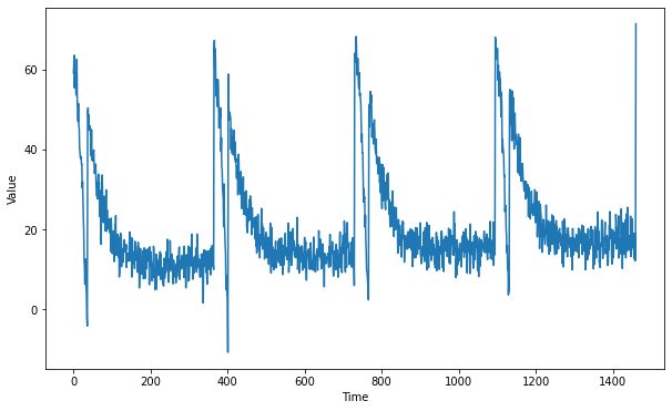
You will be generating the same time series data as in last week’s assignment.
Notice that this time all the generation is done within a function and global variables are saved within a dataclass. This is done to avoid using global scope as it was done in during the first week of the course.
If you haven’t used dataclasses before, they are just Python classes that provide a convenient syntax for storing data. You can read more about them in the docs.
def generate_time_series():
    # The time dimension or the x-coordinate of the time series
    time = np.arange(4 * 365 + 1, dtype="float32")

    # Initial series is just a straight line with a y-intercept
    y_intercept = 10
    slope = 0.005
    series = trend(time, slope) + y_intercept

    # Adding seasonality
    amplitude = 50
    series += seasonality(time, period=365, amplitude=amplitude)

    # Adding some noise
    noise_level = 3
    series += noise(time, noise_level, seed=51)

    return time, series


# Save all "global" variables within the G class (G stands for global)
@dataclass
class G:
    TIME, SERIES = generate_time_series()
    SPLIT_TIME = 1100
    WINDOW_SIZE = 20
    BATCH_SIZE = 32
    SHUFFLE_BUFFER_SIZE = 1000


# Plot the generated series
plt.figure(figsize=(10, 6))
plot_series(G.TIME, G.SERIES)
plt.show()
Processing the data
Since you already coded the train_val_split and windowed_dataset functions during past week’s assignments, this time they are provided for you:
def train_val_split(time, series, time_step=G.SPLIT_TIME):

    time_train = time[:time_step]
    series_train = series[:time_step]
    time_valid = time[time_step:]
    series_valid = series[time_step:]

    return time_train, series_train, time_valid, series_valid


# Split the dataset
time_train, series_train, time_valid, series_valid = train_val_split(G.TIME, G.SERIES)
def windowed_dataset(series, window_size=G.WINDOW_SIZE, batch_size=G.BATCH_SIZE, shuffle_buffer=G.SHUFFLE_BUFFER_SIZE):
    dataset = tf.data.Dataset.from_tensor_slices(series)
    dataset = dataset.window(window_size + 1, shift=1, drop_remainder=True)
    dataset = dataset.flat_map(lambda window: window.batch(window_size + 1))
    dataset = dataset.shuffle(shuffle_buffer)
    dataset = dataset.map(lambda window: (window[:-1], window[-1]))
    dataset = dataset.batch(batch_size).prefetch(1)
    return dataset

# Apply the transformation to the training set
dataset = windowed_dataset(series_train)
Defining the model architecture
Now that you have a function that will process the data before it is fed into your neural network for training, it is time to define you layer architecture. Unlike previous weeks or courses in which you define your layers and compile the model in the same function, here you will first need to complete the create_uncompiled_model function below.
This is done so you can reuse your model’s layers for the learning rate adjusting and the actual training.
Hint:
- Fill in the
Lambdalayers at the beginning and end of the network with the correct lamda functions. - You should use
SimpleRNNorBidirectional(LSTM)as intermediate layers. - The last layer of the network (before the last
Lambda) should be aDenselayer.
def create_uncompiled_model():

    ### START CODE HERE

    model = tf.keras.models.Sequential([
        tf.keras.layers.Lambda(lambda x: tf.expand_dims(x, axis = -1), input_shape = [G.WINDOW_SIZE]),
        tf.keras.layers.Bidirectional(
            tf.keras.layers.LSTM(64, return_sequences = True)
        ),
        tf.keras.layers.LSTM(64),
        tf.keras.layers.Dense(1),
        tf.keras.layers.Lambda(lambda x: x * 100.0)
    ])

    ### END CODE HERE

    return model
# Test your uncompiled model
uncompiled_model = create_uncompiled_model()

try:
    uncompiled_model.predict(dataset)
except:
    print("Your current architecture is incompatible with the windowed dataset, try adjusting it.")
else:
    print("Your current architecture is compatible with the windowed dataset! :)")
Your current architecture is compatible with the windowed dataset! :)
Adjusting the learning rate - (Optional Exercise)
As you saw in the lecture you can leverage Tensorflow’s callbacks to dinamically vary the learning rate during training. This can be helpful to get a better sense of which learning rate better acommodates to the problem at hand.
Notice that this is only changing the learning rate during the training process to give you an idea of what a reasonable learning rate is and should not be confused with selecting the best learning rate, this is known as hyperparameter optimization and it is outside the scope of this course.
For the optimizers you can try out:
tf.keras.optimizers.Adamtf.keras.optimizers.SGDwith a momentum of 0.9
def adjust_learning_rate():

    model = create_uncompiled_model()

    lr_schedule = tf.keras.callbacks.LearningRateScheduler(lambda epoch: 1e-6 * 10**(epoch / 20))

    ### START CODE HERE

    # Select your optimizer
    optimizer = tf.keras.optimizers.Adam()

    # Compile the model passing in the appropriate loss
    model.compile(loss="mae",
                  optimizer=optimizer,
                  metrics=["mae"])

    ### END CODE HERE

    history = model.fit(dataset, epochs=100, callbacks=[lr_schedule])

    return history
# Run the training with dynamic LR
lr_history = adjust_learning_rate()
Epoch 1/100
34/34 [==============================] - 6s 57ms/step - loss: 15.4085 - mae: 15.4085 - lr: 1.0000e-06
Epoch 2/100
34/34 [==============================] - 2s 48ms/step - loss: 14.7233 - mae: 14.7233 - lr: 1.1220e-06
Epoch 3/100
34/34 [==============================] - 2s 48ms/step - loss: 14.1353 - mae: 14.1353 - lr: 1.2589e-06
Epoch 4/100
34/34 [==============================] - 2s 48ms/step - loss: 13.6780 - mae: 13.6780 - lr: 1.4125e-06
Epoch 5/100
34/34 [==============================] - 2s 43ms/step - loss: 13.3706 - mae: 13.3706 - lr: 1.5849e-06
Epoch 6/100
34/34 [==============================] - 2s 43ms/step - loss: 13.0922 - mae: 13.0922 - lr: 1.7783e-06
Epoch 7/100
34/34 [==============================] - 2s 43ms/step - loss: 12.8041 - mae: 12.8041 - lr: 1.9953e-06
Epoch 8/100
34/34 [==============================] - 1s 40ms/step - loss: 12.4786 - mae: 12.4786 - lr: 2.2387e-06
Epoch 9/100
34/34 [==============================] - ETA: 0s - loss: 12.1186 - mae: 12.118 - 1s 39ms/step - loss: 12.1186 - mae: 12.1186 - lr: 2.5119e-06
Epoch 10/100
34/34 [==============================] - 1s 37ms/step - loss: 11.7219 - mae: 11.7219 - lr: 2.8184e-06
Epoch 11/100
34/34 [==============================] - 1s 37ms/step - loss: 11.2840 - mae: 11.2840 - lr: 3.1623e-06
Epoch 12/100
34/34 [==============================] - 1s 38ms/step - loss: 10.8001 - mae: 10.8001 - lr: 3.5481e-06
Epoch 13/100
34/34 [==============================] - 1s 37ms/step - loss: 10.2948 - mae: 10.2948 - lr: 3.9811e-06
Epoch 14/100
34/34 [==============================] - 1s 38ms/step - loss: 9.7688 - mae: 9.7688 - lr: 4.4668e-06
Epoch 15/100
34/34 [==============================] - 1s 37ms/step - loss: 9.1993 - mae: 9.1993 - lr: 5.0119e-06
Epoch 16/100
34/34 [==============================] - 1s 37ms/step - loss: 8.5852 - mae: 8.5852 - lr: 5.6234e-06
Epoch 17/100
34/34 [==============================] - 1s 37ms/step - loss: 7.9532 - mae: 7.9532 - lr: 6.3096e-06
Epoch 18/100
34/34 [==============================] - 1s 37ms/step - loss: 7.3244 - mae: 7.3244 - lr: 7.0795e-06
Epoch 19/100
34/34 [==============================] - 1s 37ms/step - loss: 6.7185 - mae: 6.7185 - lr: 7.9433e-06
Epoch 20/100
34/34 [==============================] - 1s 38ms/step - loss: 6.2461 - mae: 6.2461 - lr: 8.9125e-06
Epoch 21/100
34/34 [==============================] - 1s 37ms/step - loss: 5.8771 - mae: 5.8771 - lr: 1.0000e-05
Epoch 22/100
34/34 [==============================] - 1s 38ms/step - loss: 5.5676 - mae: 5.5676 - lr: 1.1220e-05
Epoch 23/100
34/34 [==============================] - 1s 37ms/step - loss: 5.3349 - mae: 5.3349 - lr: 1.2589e-05
Epoch 24/100
34/34 [==============================] - 1s 38ms/step - loss: 5.0971 - mae: 5.0971 - lr: 1.4125e-05
Epoch 25/100
34/34 [==============================] - 1s 38ms/step - loss: 4.8860 - mae: 4.8860 - lr: 1.5849e-05
Epoch 26/100
34/34 [==============================] - 1s 39ms/step - loss: 4.6601 - mae: 4.6601 - lr: 1.7783e-05
Epoch 27/100
34/34 [==============================] - 1s 38ms/step - loss: 4.4316 - mae: 4.4316 - lr: 1.9953e-05
Epoch 28/100
34/34 [==============================] - 1s 37ms/step - loss: 4.2357 - mae: 4.2357 - lr: 2.2387e-05
Epoch 29/100
34/34 [==============================] - 1s 38ms/step - loss: 4.0721 - mae: 4.0721 - lr: 2.5119e-05
Epoch 30/100
34/34 [==============================] - 1s 40ms/step - loss: 3.9148 - mae: 3.9148 - lr: 2.8184e-05
Epoch 31/100
34/34 [==============================] - 1s 39ms/step - loss: 3.8337 - mae: 3.8337 - lr: 3.1623e-05
Epoch 32/100
34/34 [==============================] - 1s 40ms/step - loss: 3.7628 - mae: 3.7628 - lr: 3.5481e-05
Epoch 33/100
34/34 [==============================] - 1s 39ms/step - loss: 3.7120 - mae: 3.7120 - lr: 3.9811e-05
Epoch 34/100
34/34 [==============================] - 1s 41ms/step - loss: 3.6400 - mae: 3.6400 - lr: 4.4668e-05
Epoch 35/100
34/34 [==============================] - 1s 40ms/step - loss: 3.6421 - mae: 3.6421 - lr: 5.0119e-05
Epoch 36/100
34/34 [==============================] - 1s 39ms/step - loss: 3.6420 - mae: 3.6420 - lr: 5.6234e-05
Epoch 37/100
34/34 [==============================] - 1s 38ms/step - loss: 3.6904 - mae: 3.6904 - lr: 6.3096e-05
Epoch 38/100
34/34 [==============================] - 1s 39ms/step - loss: 3.7449 - mae: 3.7449 - lr: 7.0795e-05
Epoch 39/100
34/34 [==============================] - 1s 37ms/step - loss: 3.7163 - mae: 3.7163 - lr: 7.9433e-05
Epoch 40/100
34/34 [==============================] - 1s 38ms/step - loss: 3.4900 - mae: 3.4900 - lr: 8.9125e-05
Epoch 41/100
34/34 [==============================] - 1s 38ms/step - loss: 3.5252 - mae: 3.5252 - lr: 1.0000e-04
Epoch 42/100
34/34 [==============================] - 1s 37ms/step - loss: 3.4214 - mae: 3.4214 - lr: 1.1220e-04
Epoch 43/100
34/34 [==============================] - 1s 37ms/step - loss: 3.5359 - mae: 3.5359 - lr: 1.2589e-04
Epoch 44/100
34/34 [==============================] - 1s 39ms/step - loss: 3.3118 - mae: 3.3118 - lr: 1.4125e-04
Epoch 45/100
34/34 [==============================] - 1s 37ms/step - loss: 3.4965 - mae: 3.4965 - lr: 1.5849e-04
Epoch 46/100
34/34 [==============================] - 1s 38ms/step - loss: 3.4036 - mae: 3.4036 - lr: 1.7783e-04
Epoch 47/100
34/34 [==============================] - 1s 37ms/step - loss: 3.3558 - mae: 3.3558 - lr: 1.9953e-04
Epoch 48/100
34/34 [==============================] - 1s 37ms/step - loss: 3.4253 - mae: 3.4253 - lr: 2.2387e-04
Epoch 49/100
34/34 [==============================] - 1s 37ms/step - loss: 3.3425 - mae: 3.3425 - lr: 2.5119e-04
Epoch 50/100
34/34 [==============================] - 1s 38ms/step - loss: 3.3003 - mae: 3.3003 - lr: 2.8184e-04
Epoch 51/100
34/34 [==============================] - 1s 37ms/step - loss: 3.4538 - mae: 3.4538 - lr: 3.1623e-04
Epoch 52/100
34/34 [==============================] - 1s 38ms/step - loss: 3.4858 - mae: 3.4858 - lr: 3.5481e-04
Epoch 53/100
34/34 [==============================] - 1s 37ms/step - loss: 3.4264 - mae: 3.4264 - lr: 3.9811e-04
Epoch 54/100
34/34 [==============================] - 1s 38ms/step - loss: 3.3855 - mae: 3.3855 - lr: 4.4668e-04
Epoch 55/100
34/34 [==============================] - 1s 39ms/step - loss: 3.1641 - mae: 3.1641 - lr: 5.0119e-04
Epoch 56/100
34/34 [==============================] - 1s 39ms/step - loss: 3.5491 - mae: 3.5491 - lr: 5.6234e-04
Epoch 57/100
34/34 [==============================] - 1s 41ms/step - loss: 3.8132 - mae: 3.8132 - lr: 6.3096e-04
Epoch 58/100
34/34 [==============================] - 1s 38ms/step - loss: 3.3706 - mae: 3.3706 - lr: 7.0795e-04
Epoch 59/100
34/34 [==============================] - 1s 38ms/step - loss: 4.0202 - mae: 4.0202 - lr: 7.9433e-04
Epoch 60/100
34/34 [==============================] - 1s 39ms/step - loss: 3.9237 - mae: 3.9237 - lr: 8.9125e-04
Epoch 61/100
34/34 [==============================] - 1s 38ms/step - loss: 3.2308 - mae: 3.2308 - lr: 0.0010
Epoch 62/100
34/34 [==============================] - 1s 37ms/step - loss: 3.6452 - mae: 3.6452 - lr: 0.0011
Epoch 63/100
34/34 [==============================] - 1s 38ms/step - loss: 3.1732 - mae: 3.1732 - lr: 0.0013
Epoch 64/100
34/34 [==============================] - 1s 37ms/step - loss: 3.4206 - mae: 3.4206 - lr: 0.0014
Epoch 65/100
34/34 [==============================] - 1s 37ms/step - loss: 3.1990 - mae: 3.1990 - lr: 0.0016
Epoch 66/100
34/34 [==============================] - 1s 37ms/step - loss: 3.3305 - mae: 3.3305 - lr: 0.0018
Epoch 67/100
34/34 [==============================] - 1s 38ms/step - loss: 3.2590 - mae: 3.2590 - lr: 0.0020
Epoch 68/100
34/34 [==============================] - 1s 38ms/step - loss: 3.4258 - mae: 3.4258 - lr: 0.0022
Epoch 69/100
34/34 [==============================] - 1s 39ms/step - loss: 3.5063 - mae: 3.5063 - lr: 0.0025
Epoch 70/100
34/34 [==============================] - 1s 37ms/step - loss: 3.3839 - mae: 3.3839 - lr: 0.0028
Epoch 71/100
34/34 [==============================] - 1s 38ms/step - loss: 3.0728 - mae: 3.0728 - lr: 0.0032
Epoch 72/100
34/34 [==============================] - 1s 37ms/step - loss: 3.4088 - mae: 3.4088 - lr: 0.0035
Epoch 73/100
34/34 [==============================] - 1s 38ms/step - loss: 3.4462 - mae: 3.4462 - lr: 0.0040
Epoch 74/100
34/34 [==============================] - 1s 37ms/step - loss: 3.3668 - mae: 3.3668 - lr: 0.0045
Epoch 75/100
34/34 [==============================] - 1s 37ms/step - loss: 3.6497 - mae: 3.6497 - lr: 0.0050
Epoch 76/100
34/34 [==============================] - 1s 38ms/step - loss: 3.2515 - mae: 3.2515 - lr: 0.0056
Epoch 77/100
34/34 [==============================] - 1s 37ms/step - loss: 3.3339 - mae: 3.3339 - lr: 0.0063
Epoch 78/100
34/34 [==============================] - 1s 40ms/step - loss: 3.5556 - mae: 3.5556 - lr: 0.0071
Epoch 79/100
34/34 [==============================] - 1s 39ms/step - loss: 3.3899 - mae: 3.3899 - lr: 0.0079
Epoch 80/100
34/34 [==============================] - 1s 37ms/step - loss: 4.2463 - mae: 4.2463 - lr: 0.0089
Epoch 81/100
34/34 [==============================] - 1s 38ms/step - loss: 3.3428 - mae: 3.3428 - lr: 0.0100
Epoch 82/100
34/34 [==============================] - 1s 37ms/step - loss: 3.0451 - mae: 3.0451 - lr: 0.0112
Epoch 83/100
34/34 [==============================] - 1s 37ms/step - loss: 3.9983 - mae: 3.9983 - lr: 0.0126
Epoch 84/100
34/34 [==============================] - 1s 37ms/step - loss: 3.2463 - mae: 3.2463 - lr: 0.0141
Epoch 85/100
34/34 [==============================] - 1s 37ms/step - loss: 3.1193 - mae: 3.1193 - lr: 0.0158
Epoch 86/100
34/34 [==============================] - 1s 37ms/step - loss: 3.5554 - mae: 3.5554 - lr: 0.0178
Epoch 87/100
34/34 [==============================] - 1s 38ms/step - loss: 3.4603 - mae: 3.4603 - lr: 0.0200
Epoch 88/100
34/34 [==============================] - 1s 37ms/step - loss: 3.1508 - mae: 3.1508 - lr: 0.0224
Epoch 89/100
34/34 [==============================] - 1s 38ms/step - loss: 3.1286 - mae: 3.1286 - lr: 0.0251
Epoch 90/100
34/34 [==============================] - 1s 39ms/step - loss: 3.1420 - mae: 3.1420 - lr: 0.0282
Epoch 91/100
34/34 [==============================] - 1s 40ms/step - loss: 3.2516 - mae: 3.2516 - lr: 0.0316
Epoch 92/100
34/34 [==============================] - 1s 40ms/step - loss: 3.2258 - mae: 3.2258 - lr: 0.0355
Epoch 93/100
34/34 [==============================] - 1s 38ms/step - loss: 3.3116 - mae: 3.3116 - lr: 0.0398
Epoch 94/100
34/34 [==============================] - 1s 38ms/step - loss: 3.5323 - mae: 3.5323 - lr: 0.0447
Epoch 95/100
34/34 [==============================] - 1s 38ms/step - loss: 3.4423 - mae: 3.4423 - lr: 0.0501
Epoch 96/100
34/34 [==============================] - 1s 39ms/step - loss: 3.6105 - mae: 3.6105 - lr: 0.0562
Epoch 97/100
34/34 [==============================] - 1s 39ms/step - loss: 3.4228 - mae: 3.4228 - lr: 0.0631
Epoch 98/100
34/34 [==============================] - 1s 40ms/step - loss: 3.8440 - mae: 3.8440 - lr: 0.0708
Epoch 99/100
34/34 [==============================] - 1s 40ms/step - loss: 3.5850 - mae: 3.5850 - lr: 0.0794
Epoch 100/100
34/34 [==============================] - 1s 40ms/step - loss: 3.7424 - mae: 3.7424 - lr: 0.0891
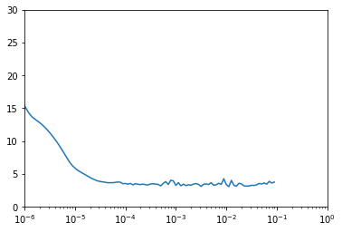
# Plot the loss for every LR
plt.semilogx(lr_history.history["lr"], lr_history.history["loss"])
plt.axis([1e-6, 1, 0, 30])
(1e-06, 1.0, 0.0, 30.0)
Compiling the model
Now that you have trained the model while varying the learning rate, it is time to do the actual training that will be used to forecast the time series. For this complete the create_model function below.
Notice that you are reusing the architecture you defined in the create_uncompiled_model earlier. Now you only need to compile this model using the appropriate loss, optimizer (and learning rate).
Hint:
-
The training should be really quick so if you notice that each epoch is taking more than a few seconds, consider trying a different architecture.
-
If after the first epoch you get an output like this:
loss: nan - mae: nanit is very likely that your network is suffering from exploding gradients. This is a common problem if you usedSGDas optimizer and set a learning rate that is too high. If you encounter this problem consider lowering the learning rate or using Adam with the default learning rate.
def create_model():

    tf.random.set_seed(51)

    model = create_uncompiled_model()

    ### START CODE HERE

    model.compile(loss="mae",
                  optimizer=tf.keras.optimizers.Adam(),
                  metrics=["mae"])

    ### END CODE HERE

    return model
# Save an instance of the model
model = create_model()

# Train it
history = model.fit(dataset, epochs=50)
Epoch 1/50
34/34 [==============================] - 6s 56ms/step - loss: 7.5805 - mae: 7.5805
Epoch 2/50
34/34 [==============================] - 2s 45ms/step - loss: 3.7207 - mae: 3.7207
Epoch 3/50
34/34 [==============================] - 2s 44ms/step - loss: 3.7665 - mae: 3.7665
Epoch 4/50
34/34 [==============================] - 2s 45ms/step - loss: 3.5993 - mae: 3.5993
Epoch 5/50
34/34 [==============================] - 2s 45ms/step - loss: 4.1945 - mae: 4.1945
Epoch 6/50
34/34 [==============================] - 2s 43ms/step - loss: 4.3349 - mae: 4.3349
Epoch 7/50
34/34 [==============================] - 2s 44ms/step - loss: 3.3802 - mae: 3.3802
Epoch 8/50
34/34 [==============================] - 2s 44ms/step - loss: 3.2149 - mae: 3.2149
Epoch 9/50
34/34 [==============================] - 2s 44ms/step - loss: 3.2508 - mae: 3.2508
Epoch 10/50
34/34 [==============================] - 1s 40ms/step - loss: 3.0986 - mae: 3.0986
Epoch 11/50
34/34 [==============================] - 1s 41ms/step - loss: 3.3968 - mae: 3.3968
Epoch 12/50
34/34 [==============================] - 1s 39ms/step - loss: 3.1662 - mae: 3.1662
Epoch 13/50
34/34 [==============================] - 1s 38ms/step - loss: 3.2600 - mae: 3.2600
Epoch 14/50
34/34 [==============================] - 1s 38ms/step - loss: 3.0739 - mae: 3.0739
Epoch 15/50
34/34 [==============================] - 1s 38ms/step - loss: 3.1872 - mae: 3.1872
Epoch 16/50
34/34 [==============================] - 1s 38ms/step - loss: 3.0427 - mae: 3.0427
Epoch 17/50
34/34 [==============================] - 1s 38ms/step - loss: 3.1703 - mae: 3.1703
Epoch 18/50
34/34 [==============================] - 1s 39ms/step - loss: 3.3530 - mae: 3.3530
Epoch 19/50
34/34 [==============================] - 1s 38ms/step - loss: 3.0865 - mae: 3.0865
Epoch 20/50
34/34 [==============================] - 1s 39ms/step - loss: 3.0929 - mae: 3.0929
Epoch 21/50
34/34 [==============================] - 1s 37ms/step - loss: 3.2252 - mae: 3.2252
Epoch 22/50
34/34 [==============================] - 1s 38ms/step - loss: 3.0056 - mae: 3.0056
Epoch 23/50
34/34 [==============================] - 1s 36ms/step - loss: 3.0569 - mae: 3.0569
Epoch 24/50
34/34 [==============================] - 1s 37ms/step - loss: 3.2279 - mae: 3.2279
Epoch 25/50
34/34 [==============================] - 1s 38ms/step - loss: 3.1595 - mae: 3.1595
Epoch 26/50
34/34 [==============================] - 1s 39ms/step - loss: 3.0330 - mae: 3.0330
Epoch 27/50
34/34 [==============================] - 1s 37ms/step - loss: 2.9198 - mae: 2.9198
Epoch 28/50
34/34 [==============================] - 1s 37ms/step - loss: 3.1339 - mae: 3.1339
Epoch 29/50
34/34 [==============================] - 1s 37ms/step - loss: 3.1329 - mae: 3.1329
Epoch 30/50
34/34 [==============================] - 1s 37ms/step - loss: 3.0699 - mae: 3.0699
Epoch 31/50
34/34 [==============================] - 1s 39ms/step - loss: 3.2925 - mae: 3.2925
Epoch 32/50
34/34 [==============================] - 1s 37ms/step - loss: 3.1318 - mae: 3.1318
Epoch 33/50
34/34 [==============================] - 1s 38ms/step - loss: 3.0300 - mae: 3.0300
Epoch 34/50
34/34 [==============================] - 1s 37ms/step - loss: 2.9795 - mae: 2.9795
Epoch 35/50
34/34 [==============================] - 1s 38ms/step - loss: 2.9426 - mae: 2.9426
Epoch 36/50
34/34 [==============================] - 1s 39ms/step - loss: 2.9190 - mae: 2.9190
Epoch 37/50
34/34 [==============================] - 1s 37ms/step - loss: 2.9501 - mae: 2.9501
Epoch 38/50
34/34 [==============================] - 1s 37ms/step - loss: 3.0247 - mae: 3.0247
Epoch 39/50
34/34 [==============================] - 1s 37ms/step - loss: 2.9384 - mae: 2.9384
Epoch 40/50
34/34 [==============================] - 1s 37ms/step - loss: 2.8566 - mae: 2.8566
Epoch 41/50
34/34 [==============================] - 1s 37ms/step - loss: 2.9794 - mae: 2.9794
Epoch 42/50
34/34 [==============================] - 1s 38ms/step - loss: 3.2196 - mae: 3.2196
Epoch 43/50
34/34 [==============================] - 1s 37ms/step - loss: 2.9570 - mae: 2.9570
Epoch 44/50
34/34 [==============================] - 1s 38ms/step - loss: 2.8551 - mae: 2.8551
Epoch 45/50
34/34 [==============================] - 1s 37ms/step - loss: 3.2549 - mae: 3.2549
Epoch 46/50
34/34 [==============================] - 1s 39ms/step - loss: 3.1121 - mae: 3.1121
Epoch 47/50
34/34 [==============================] - 1s 39ms/step - loss: 2.8880 - mae: 2.8880
Epoch 48/50
34/34 [==============================] - 1s 37ms/step - loss: 2.9298 - mae: 2.9298
Epoch 49/50
34/34 [==============================] - 1s 38ms/step - loss: 2.9615 - mae: 2.9615
Epoch 50/50
34/34 [==============================] - 1s 38ms/step - loss: 3.0155 - mae: 3.0155
Evaluating the forecast
Now it is time to evaluate the performance of the forecast. For this you can use the compute_metrics function that you coded in a previous assignment:
def compute_metrics(true_series, forecast):

    mse = tf.keras.metrics.mean_squared_error(true_series, forecast).numpy()
    mae = tf.keras.metrics.mean_absolute_error(true_series, forecast).numpy()

    return mse, mae
At this point only the model that will perform the forecast is ready but you still need to compute the actual forecast.
Faster model forecasts
In the previous week you used a for loop to compute the forecasts for every point in the sequence. This approach is valid but there is a more efficient way of doing the same thing by using batches of data. The code to implement this is provided in the model_forecast below. Notice that the code is very similar to the one in the windowed_dataset function with the differences that:
- The dataset is windowed using
window_sizerather thanwindow_size + 1 - No shuffle should be used
- No need to split the data into features and labels
- A model is used to predict batches of the dataset
def model_forecast(model, series, window_size):
    ds = tf.data.Dataset.from_tensor_slices(series)
    ds = ds.window(window_size, shift=1, drop_remainder=True)
    ds = ds.flat_map(lambda w: w.batch(window_size))
    ds = ds.batch(32).prefetch(1)
    forecast = model.predict(ds)
    return forecast
# Compute the forecast for all the series
rnn_forecast = model_forecast(model, G.SERIES, G.WINDOW_SIZE).squeeze()

# Slice the forecast to get only the predictions for the validation set
rnn_forecast = rnn_forecast[G.SPLIT_TIME - G.WINDOW_SIZE:-1]

# Plot it
plt.figure(figsize=(10, 6))

plot_series(time_valid, series_valid)
plot_series(time_valid, rnn_forecast)
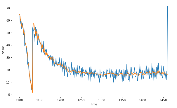
Expected Output:
A series similar to this one:

mse, mae = compute_metrics(series_valid, rnn_forecast)

print(f"mse: {mse:.2f}, mae: {mae:.2f} for forecast")
mse: 27.92, mae: 3.06 for forecast
To pass this assignment your forecast should achieve an MAE of 4.5 or less.
-
If your forecast didn’t achieve this threshold try re-training your model with a different architecture (you will need to re-run both
create_uncompiled_modelandcreate_modelfunctions) or tweaking the optimizer’s parameters. -
If your forecast did achieve this threshold run the following cell to save your model in a
tarfile which will be used for grading and after doing so, submit your assigment for grading. -
This environment includes a dummy
SavedModeldirectory which contains a dummy model trained for one epoch. To replace this file with your actual model you need to run the next cell before submitting for grading. -
Unlike last week, this time the model is saved using the
SavedModelformat. This is done because the HDF5 format does not fully supportLambdalayers.
# Save your model in the SavedModel format
model.save('saved_model/my_model')

# Compress the directory using tar
! tar -czvf saved_model.tar.gz saved_model/
INFO:tensorflow:Assets written to: saved_model/my_model/assets


INFO:tensorflow:Assets written to: saved_model/my_model/assets


saved_model/
saved_model/my_model/
saved_model/my_model/keras_metadata.pb
saved_model/my_model/variables/
saved_model/my_model/variables/variables.data-00000-of-00001
saved_model/my_model/variables/variables.index
saved_model/my_model/saved_model.pb
saved_model/my_model/assets/
Congratulations on finishing this week’s assignment!
You have successfully implemented a neural network capable of forecasting time series leveraging Tensorflow’s layers for sequence modelling such as RNNs and LSTMs! This resulted in a forecast that matches (or even surpasses) the one from last week while training for half of the epochs.
Keep it up!
Please click here if you want to experiment with any of the non-graded code.
Important Note: Please only do this when you've already passed the assignment to avoid problems with the autograder.
- On the notebook’s menu, click “View” > “Cell Toolbar” > “Edit Metadata”
- Hit the “Edit Metadata” button next to the code cell which you want to lock/unlock
- Set the attribute value for “editable” to:
- “true” if you want to unlock it
- “false” if you want to lock it
- On the notebook’s menu, click “View” > “Cell Toolbar” > “None”
Here's a short demo of how to do the steps above: