Coursera

Week 4: Using real world data

Welcome! So far you have worked exclusively with generated data. This time you will be using the Daily Minimum Temperatures in Melbourne dataset which contains data of the daily minimum temperatures recorded in Melbourne from 1981 to 1990. In addition to be using Tensorflow’s layers for processing sequence data such as Recurrent layers or LSTMs you will also use Convolutional layers to improve the model’s performance.

Let’s get started!

NOTE: To prevent errors from the autograder, you are not allowed to edit or delete some of the cells in this notebook . Please only put your solutions in between the ### START CODE HERE and ### END CODE HERE code comments, and also refrain from adding any new cells. Once you have passed this assignment and want to experiment with any of the locked cells, you may follow the instructions at the bottom of this notebook.

import csv
import pickle
import numpy as np
import tensorflow as tf
import matplotlib.pyplot as plt
from dataclasses import dataclass
from absl import logging
logging.set_verbosity(logging.ERROR)

Begin by looking at the structure of the csv that contains the data:

TEMPERATURES_CSV = './data/daily-min-temperatures.csv'

with open(TEMPERATURES_CSV, 'r') as csvfile:
    print(f"Header looks like this:\n\n{csvfile.readline()}")    
    print(f"First data point looks like this:\n\n{csvfile.readline()}")
    print(f"Second data point looks like this:\n\n{csvfile.readline()}")

Header looks like this:

"Date","Temp"

First data point looks like this:

"1981-01-01",20.7

Second data point looks like this:

"1981-01-02",17.9

As you can see, each data point is composed of the date and the recorded minimum temperature for that date.

In the first exercise you will code a function to read the data from the csv but for now run the next cell to load a helper function to plot the time series.

def plot_series(time, series, format="-", start=0, end=None):
    plt.plot(time[start:end], series[start:end], format)
    plt.xlabel("Time")
    plt.ylabel("Value")
    plt.grid(True)

Parsing the raw data

Now you need to read the data from the csv file. To do so, complete the parse_data_from_file function.

A couple of things to note:

• You should omit the first line as the file contains headers.
• There is no need to save the data points as numpy arrays, regular lists is fine.
• To read from csv files use csv.reader by passing the appropriate arguments.
• csv.reader returns an iterable that returns each row in every iteration. So the temperature can be accessed via row[1] and the date can be discarded.
• The times list should contain every timestep (starting at zero), which is just a sequence of ordered numbers with the same length as the temperatures list.
• The values of the temperatures should be of float type. You can use Python’s built-in float function to ensure this.

def parse_data_from_file(filename):
    
    times = []
    temperatures = []

    with open(filename) as csvfile:
        
        ### START CODE HERE
        
        reader = csv.reader(csvfile, delimiter=",")
        next(reader)
        
        for row in reader:
            times.append(row[0])
            temperatures.append(float(row[1]))
        ### END CODE HERE
            
    return times, temperatures

The next cell will use your function to compute the times and temperatures and will save these as numpy arrays within the G dataclass. This cell will also plot the time series:

# Test your function and save all "global" variables within the G class (G stands for global)
@dataclass
class G:
    TEMPERATURES_CSV = './data/daily-min-temperatures.csv'
    times, temperatures = parse_data_from_file(TEMPERATURES_CSV)
    TIME = np.array(times)
    SERIES = np.array(temperatures)
    SPLIT_TIME = 2500
    WINDOW_SIZE = 64
    BATCH_SIZE = 32
    SHUFFLE_BUFFER_SIZE = 1000


plt.figure(figsize=(10, 6))
plot_series(G.TIME, G.SERIES)
plt.show()

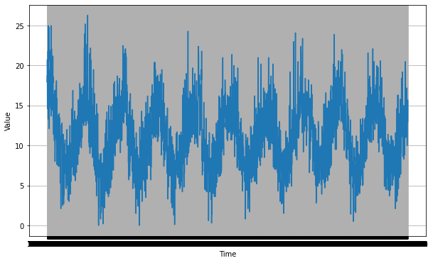
Expected Output:

Processing the data

Since you already coded the train_val_split and windowed_dataset functions during past week’s assignments, this time they are provided for you:

def train_val_split(time, series, time_step=G.SPLIT_TIME):

    time_train = time[:time_step]
    series_train = series[:time_step]
    time_valid = time[time_step:]
    series_valid = series[time_step:]

    return time_train, series_train, time_valid, series_valid


# Split the dataset
time_train, series_train, time_valid, series_valid = train_val_split(G.TIME, G.SERIES)

def windowed_dataset(series, window_size=G.WINDOW_SIZE, batch_size=G.BATCH_SIZE, shuffle_buffer=G.SHUFFLE_BUFFER_SIZE):
    ds = tf.data.Dataset.from_tensor_slices(series)
    ds = ds.window(window_size + 1, shift=1, drop_remainder=True)
    ds = ds.flat_map(lambda w: w.batch(window_size + 1))
    ds = ds.shuffle(shuffle_buffer)
    ds = ds.map(lambda w: (w[:-1], w[-1]))
    ds = ds.batch(batch_size).prefetch(1)
    return ds


# Apply the transformation to the training set
train_set = windowed_dataset(series_train, window_size=G.WINDOW_SIZE, batch_size=G.BATCH_SIZE, shuffle_buffer=G.SHUFFLE_BUFFER_SIZE)

Defining the model architecture

Now that you have a function that will process the data before it is fed into your neural network for training, it is time to define your layer architecture. Just as in last week’s assignment you will do the layer definition and compilation in two separate steps. Begin by completing the create_uncompiled_model function below.

This is done so you can reuse your model’s layers for the learning rate adjusting and the actual training.

Hint:

• Lambda layers are not required.
• Use a combination of Conv1D and LSTM layers followed by Dense layers

def create_uncompiled_model():

    ### START CODE HERE
    
    model = tf.keras.models.Sequential([
        tf.keras.layers.Conv1D(filters=64, kernel_size=3,
                      strides=1,
                      activation="relu",
                      padding='causal',
                      input_shape=[None, 1]),
        tf.keras.layers.LSTM(64, return_sequences=True),
        tf.keras.layers.LSTM(64),
        tf.keras.layers.Dense(30, activation="relu"),
        tf.keras.layers.Dense(10, activation="relu"),
        tf.keras.layers.Dense(1),
    ]) 
    
    ### END CODE HERE

    return model

You can test your model with the code below. If you get an error, it’s likely that your model is returning a sequence. You can indeed use an LSTM with return_sequences=True but you have to feed it into another layer that generates a single prediction. You can review the lectures or the previous ungraded labs to see how that is done.

# Test your uncompiled model

# Create an instance of the model
uncompiled_model = create_uncompiled_model()

# Get one batch of the training set(X = input, y = label)
for X, y in train_set.take(1):
    
    # Generate a prediction
    print(f'Testing model prediction with input of shape {X.shape}...')
    y_pred = uncompiled_model.predict(X)
    
# Compare the shape of the prediction and the label y (remove dimensions of size 1)
y_pred_shape = y_pred.squeeze().shape

assert y_pred_shape == y.shape, (f'Squeezed predicted y shape = {y_pred_shape} '
                                           f'whereas actual y shape = {y.shape}.')

print("Your current architecture is compatible with the windowed dataset! :)")

Testing model prediction with input of shape (32, 64)...
Your current architecture is compatible with the windowed dataset! :)

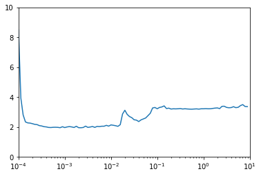
Adjusting the learning rate - (Optional Exercise)

As you saw in the lectures, you can leverage Tensorflow’s callbacks to dynamically vary the learning rate before doing the actual training. This can be helpful in finding what value works best with your model. Note that this is only one way of finding the best learning rate. There are other techniques for hyperparameter optimization but it is outside the scope of this course.

For the optimizers you can try out:

• tf.keras.optimizers.Adam
• tf.keras.optimizers.SGD with a momentum of 0.9

def adjust_learning_rate(dataset):
    
    model = create_uncompiled_model()
    
    lr_schedule = tf.keras.callbacks.LearningRateScheduler(lambda epoch: 1e-4 * 10**(epoch / 20))
    
    ### START CODE HERE
    
    # Select your optimizer
    optimizer = tf.keras.optimizers.Adam()
    
    # Compile the model passing in the appropriate loss
    model.compile(loss="mae",
                  optimizer=optimizer, 
                  metrics=["mae"]) 
    
    ### END CODE HERE
    
    history = model.fit(dataset, epochs=100, callbacks=[lr_schedule])
    
    return history

# Run the training with dynamic LR
lr_history = adjust_learning_rate(train_set)

Epoch 1/100
77/77 [==============================] - 10s 90ms/step - loss: 8.4831 - mae: 8.4831 - lr: 1.0000e-04
Epoch 2/100
77/77 [==============================] - 8s 98ms/step - loss: 3.9307 - mae: 3.9307 - lr: 1.1220e-04
Epoch 3/100
77/77 [==============================] - 7s 93ms/step - loss: 2.7955 - mae: 2.7955 - lr: 1.2589e-04
Epoch 4/100
77/77 [==============================] - 7s 93ms/step - loss: 2.3296 - mae: 2.3296 - lr: 1.4125e-04
Epoch 5/100
77/77 [==============================] - 8s 99ms/step - loss: 2.2657 - mae: 2.2657 - lr: 1.5849e-04
Epoch 6/100
77/77 [==============================] - 8s 102ms/step - loss: 2.2510 - mae: 2.2510 - lr: 1.7783e-04
Epoch 7/100
77/77 [==============================] - 7s 94ms/step - loss: 2.2138 - mae: 2.2138 - lr: 1.9953e-04
Epoch 8/100
77/77 [==============================] - 7s 94ms/step - loss: 2.1673 - mae: 2.1673 - lr: 2.2387e-04
Epoch 9/100
77/77 [==============================] - 7s 89ms/step - loss: 2.1519 - mae: 2.1519 - lr: 2.5119e-04
Epoch 10/100
77/77 [==============================] - 7s 93ms/step - loss: 2.0838 - mae: 2.0838 - lr: 2.8184e-04
Epoch 11/100
77/77 [==============================] - 7s 93ms/step - loss: 2.0601 - mae: 2.0601 - lr: 3.1623e-04
Epoch 12/100
77/77 [==============================] - 7s 92ms/step - loss: 2.0122 - mae: 2.0122 - lr: 3.5481e-04
Epoch 13/100
77/77 [==============================] - 7s 95ms/step - loss: 1.9967 - mae: 1.9967 - lr: 3.9811e-04
Epoch 14/100
77/77 [==============================] - 7s 93ms/step - loss: 1.9609 - mae: 1.9609 - lr: 4.4668e-04
Epoch 15/100
77/77 [==============================] - 7s 96ms/step - loss: 1.9556 - mae: 1.9556 - lr: 5.0119e-04
Epoch 16/100
77/77 [==============================] - 7s 94ms/step - loss: 1.9703 - mae: 1.9703 - lr: 5.6234e-04
Epoch 17/100
77/77 [==============================] - 7s 90ms/step - loss: 1.9732 - mae: 1.9732 - lr: 6.3096e-04
Epoch 18/100
77/77 [==============================] - 7s 91ms/step - loss: 1.9667 - mae: 1.9667 - lr: 7.0795e-04
Epoch 19/100
77/77 [==============================] - 7s 90ms/step - loss: 1.9448 - mae: 1.9448 - lr: 7.9433e-04
Epoch 20/100
77/77 [==============================] - 7s 89ms/step - loss: 2.0086 - mae: 2.0086 - lr: 8.9125e-04
Epoch 21/100
77/77 [==============================] - 7s 92ms/step - loss: 1.9521 - mae: 1.9521 - lr: 0.0010
Epoch 22/100
77/77 [==============================] - 8s 99ms/step - loss: 1.9937 - mae: 1.9937 - lr: 0.0011
Epoch 23/100
77/77 [==============================] - 7s 89ms/step - loss: 2.0178 - mae: 2.0178 - lr: 0.0013
Epoch 24/100
77/77 [==============================] - 7s 90ms/step - loss: 1.9958 - mae: 1.9958 - lr: 0.0014
Epoch 25/100
77/77 [==============================] - 7s 86ms/step - loss: 1.9573 - mae: 1.9573 - lr: 0.0016
Epoch 26/100
77/77 [==============================] - 7s 85ms/step - loss: 2.0402 - mae: 2.0402 - lr: 0.0018
Epoch 27/100
77/77 [==============================] - 7s 94ms/step - loss: 1.9443 - mae: 1.9443 - lr: 0.0020
Epoch 28/100
77/77 [==============================] - 8s 99ms/step - loss: 1.9410 - mae: 1.9410 - lr: 0.0022
Epoch 29/100
77/77 [==============================] - 8s 105ms/step - loss: 1.9586 - mae: 1.9586 - lr: 0.0025
Epoch 30/100
77/77 [==============================] - 8s 103ms/step - loss: 2.0487 - mae: 2.0487 - lr: 0.0028
Epoch 31/100
77/77 [==============================] - 7s 95ms/step - loss: 1.9644 - mae: 1.9644 - lr: 0.0032
Epoch 32/100
77/77 [==============================] - 7s 93ms/step - loss: 1.9890 - mae: 1.9890 - lr: 0.0035
Epoch 33/100
77/77 [==============================] - 7s 92ms/step - loss: 2.0241 - mae: 2.0241 - lr: 0.0040
Epoch 34/100
77/77 [==============================] - 7s 95ms/step - loss: 1.9648 - mae: 1.9648 - lr: 0.0045
Epoch 35/100
77/77 [==============================] - 7s 91ms/step - loss: 2.0298 - mae: 2.0298 - lr: 0.0050
Epoch 36/100
77/77 [==============================] - 7s 95ms/step - loss: 2.0174 - mae: 2.0174 - lr: 0.0056
Epoch 37/100
77/77 [==============================] - 7s 95ms/step - loss: 2.0428 - mae: 2.0428 - lr: 0.0063
Epoch 38/100
77/77 [==============================] - 7s 88ms/step - loss: 2.0425 - mae: 2.0425 - lr: 0.0071
Epoch 39/100
77/77 [==============================] - 7s 95ms/step - loss: 2.1012 - mae: 2.1012 - lr: 0.0079
Epoch 40/100
77/77 [==============================] - 7s 93ms/step - loss: 2.0486 - mae: 2.0486 - lr: 0.0089
Epoch 41/100
77/77 [==============================] - 7s 93ms/step - loss: 2.1298 - mae: 2.1298 - lr: 0.0100
Epoch 42/100
77/77 [==============================] - 7s 97ms/step - loss: 2.1062 - mae: 2.1062 - lr: 0.0112
Epoch 43/100
77/77 [==============================] - 8s 108ms/step - loss: 2.0762 - mae: 2.0762 - lr: 0.0126
Epoch 44/100
77/77 [==============================] - 7s 94ms/step - loss: 2.0354 - mae: 2.0354 - lr: 0.0141
Epoch 45/100
77/77 [==============================] - 8s 98ms/step - loss: 2.1448 - mae: 2.1448 - lr: 0.0158
Epoch 46/100
77/77 [==============================] - 7s 96ms/step - loss: 2.8612 - mae: 2.8612 - lr: 0.0178
Epoch 47/100
77/77 [==============================] - 8s 98ms/step - loss: 3.1111 - mae: 3.1111 - lr: 0.0200
Epoch 48/100
77/77 [==============================] - 8s 100ms/step - loss: 2.8357 - mae: 2.8357 - lr: 0.0224
Epoch 49/100
77/77 [==============================] - 7s 96ms/step - loss: 2.6902 - mae: 2.6902 - lr: 0.0251
Epoch 50/100
77/77 [==============================] - 7s 95ms/step - loss: 2.6150 - mae: 2.6150 - lr: 0.0282
Epoch 51/100
77/77 [==============================] - 7s 95ms/step - loss: 2.4746 - mae: 2.4746 - lr: 0.0316
Epoch 52/100
77/77 [==============================] - 7s 93ms/step - loss: 2.4510 - mae: 2.4510 - lr: 0.0355
Epoch 53/100
77/77 [==============================] - 8s 99ms/step - loss: 2.3541 - mae: 2.3541 - lr: 0.0398
Epoch 54/100
77/77 [==============================] - 7s 95ms/step - loss: 2.4671 - mae: 2.4671 - lr: 0.0447
Epoch 55/100
77/77 [==============================] - 8s 97ms/step - loss: 2.5296 - mae: 2.5296 - lr: 0.0501
Epoch 56/100
77/77 [==============================] - 7s 94ms/step - loss: 2.5931 - mae: 2.5931 - lr: 0.0562
Epoch 57/100
77/77 [==============================] - 8s 99ms/step - loss: 2.7488 - mae: 2.7488 - lr: 0.0631
Epoch 58/100
77/77 [==============================] - 7s 96ms/step - loss: 2.9090 - mae: 2.9090 - lr: 0.0708
Epoch 59/100
77/77 [==============================] - 8s 98ms/step - loss: 3.2632 - mae: 3.2632 - lr: 0.0794
Epoch 60/100
77/77 [==============================] - 7s 93ms/step - loss: 3.2961 - mae: 3.2961 - lr: 0.0891
Epoch 61/100
77/77 [==============================] - 8s 98ms/step - loss: 3.2125 - mae: 3.2125 - lr: 0.1000
Epoch 62/100
77/77 [==============================] - 7s 92ms/step - loss: 3.2983 - mae: 3.2983 - lr: 0.1122
Epoch 63/100
77/77 [==============================] - 8s 97ms/step - loss: 3.3317 - mae: 3.3317 - lr: 0.1259
Epoch 64/100
77/77 [==============================] - 7s 92ms/step - loss: 3.4019 - mae: 3.4019 - lr: 0.1413
Epoch 65/100
77/77 [==============================] - 7s 95ms/step - loss: 3.2241 - mae: 3.2241 - lr: 0.1585
Epoch 66/100
77/77 [==============================] - 7s 97ms/step - loss: 3.2513 - mae: 3.2513 - lr: 0.1778
Epoch 67/100
77/77 [==============================] - 7s 94ms/step - loss: 3.1915 - mae: 3.1915 - lr: 0.1995
Epoch 68/100
77/77 [==============================] - 7s 92ms/step - loss: 3.2079 - mae: 3.2079 - lr: 0.2239
Epoch 69/100
77/77 [==============================] - 7s 92ms/step - loss: 3.2022 - mae: 3.2022 - lr: 0.2512
Epoch 70/100
77/77 [==============================] - 7s 93ms/step - loss: 3.2099 - mae: 3.2099 - lr: 0.2818
Epoch 71/100
77/77 [==============================] - 7s 94ms/step - loss: 3.2238 - mae: 3.2238 - lr: 0.3162
Epoch 72/100
77/77 [==============================] - 8s 105ms/step - loss: 3.1942 - mae: 3.1942 - lr: 0.3548
Epoch 73/100
77/77 [==============================] - 7s 95ms/step - loss: 3.2103 - mae: 3.2103 - lr: 0.3981
Epoch 74/100
77/77 [==============================] - 7s 95ms/step - loss: 3.1958 - mae: 3.1958 - lr: 0.4467
Epoch 75/100
77/77 [==============================] - 7s 93ms/step - loss: 3.1866 - mae: 3.1866 - lr: 0.5012
Epoch 76/100
77/77 [==============================] - 8s 107ms/step - loss: 3.1832 - mae: 3.1832 - lr: 0.5623
Epoch 77/100
77/77 [==============================] - 8s 106ms/step - loss: 3.1935 - mae: 3.1935 - lr: 0.6310
Epoch 78/100
77/77 [==============================] - 7s 96ms/step - loss: 3.2024 - mae: 3.2024 - lr: 0.7079
Epoch 79/100
77/77 [==============================] - 7s 96ms/step - loss: 3.1856 - mae: 3.1856 - lr: 0.7943
Epoch 80/100
77/77 [==============================] - 7s 93ms/step - loss: 3.2083 - mae: 3.2083 - lr: 0.8913
Epoch 81/100
77/77 [==============================] - 8s 103ms/step - loss: 3.2097 - mae: 3.2097 - lr: 1.0000
Epoch 82/100
77/77 [==============================] - 7s 95ms/step - loss: 3.2196 - mae: 3.2196 - lr: 1.1220
Epoch 83/100
77/77 [==============================] - 7s 96ms/step - loss: 3.2087 - mae: 3.2087 - lr: 1.2589
Epoch 84/100
77/77 [==============================] - 8s 98ms/step - loss: 3.2122 - mae: 3.2122 - lr: 1.4125
Epoch 85/100
77/77 [==============================] - 8s 99ms/step - loss: 3.2326 - mae: 3.2326 - lr: 1.5849
Epoch 86/100
77/77 [==============================] - 8s 97ms/step - loss: 3.2545 - mae: 3.2545 - lr: 1.7783
Epoch 87/100
77/77 [==============================] - 7s 96ms/step - loss: 3.2673 - mae: 3.2673 - lr: 1.9953
Epoch 88/100
77/77 [==============================] - 8s 97ms/step - loss: 3.2206 - mae: 3.2206 - lr: 2.2387
Epoch 89/100
77/77 [==============================] - 7s 95ms/step - loss: 3.3718 - mae: 3.3718 - lr: 2.5119
Epoch 90/100
77/77 [==============================] - 8s 100ms/step - loss: 3.3792 - mae: 3.3792 - lr: 2.8184
Epoch 91/100
77/77 [==============================] - 7s 94ms/step - loss: 3.3000 - mae: 3.3000 - lr: 3.1623
Epoch 92/100
77/77 [==============================] - 7s 95ms/step - loss: 3.2771 - mae: 3.2771 - lr: 3.5481
Epoch 93/100
77/77 [==============================] - 7s 95ms/step - loss: 3.2886 - mae: 3.2886 - lr: 3.9811
Epoch 94/100
77/77 [==============================] - 7s 95ms/step - loss: 3.3493 - mae: 3.3493 - lr: 4.4668
Epoch 95/100
77/77 [==============================] - 8s 98ms/step - loss: 3.2837 - mae: 3.2837 - lr: 5.0119
Epoch 96/100
77/77 [==============================] - 8s 102ms/step - loss: 3.3061 - mae: 3.3061 - lr: 5.6234
Epoch 97/100
77/77 [==============================] - 7s 94ms/step - loss: 3.4210 - mae: 3.4210 - lr: 6.3096
Epoch 98/100
77/77 [==============================] - 7s 93ms/step - loss: 3.4878 - mae: 3.4878 - lr: 7.0795
Epoch 99/100
77/77 [==============================] - 7s 95ms/step - loss: 3.3622 - mae: 3.3622 - lr: 7.9433
Epoch 100/100
77/77 [==============================] - 7s 96ms/step - loss: 3.3557 - mae: 3.3557 - lr: 8.9125

plt.semilogx(lr_history.history["lr"], lr_history.history["loss"])
plt.axis([1e-4, 10, 0, 10])

(0.0001, 10.0, 0.0, 10.0)

Compiling the model

Now that you have trained the model while varying the learning rate, it is time to do the actual training that will be used to forecast the time series. For this complete the create_model function below.

Notice that you are reusing the architecture you defined in the create_uncompiled_model earlier. Now you only need to compile this model using the appropriate loss, optimizer (and learning rate).

Hints:

• The training should be really quick so if you notice that each epoch is taking more than a few seconds, consider trying a different architecture.

• If after the first epoch you get an output like this: loss: nan - mae: nan it is very likely that your network is suffering from exploding gradients. This is a common problem if you used SGD as optimizer and set a learning rate that is too high. If you encounter this problem consider lowering the learning rate or using Adam with the default learning rate.

def create_model():

    
    model = create_uncompiled_model()

    ### START CODE HERE

    model.compile(loss="mae",
                  optimizer=tf.keras.optimizers.Adam(learning_rate=1e-3),
                  metrics=["mae"])  
    

    ### END CODE HERE

    return model

# Save an instance of the model
model = create_model()

# Train it
history = model.fit(train_set, epochs=50)

Epoch 1/50
77/77 [==============================] - 10s 95ms/step - loss: 4.0282 - mae: 4.0282
Epoch 2/50
77/77 [==============================] - 8s 98ms/step - loss: 2.3046 - mae: 2.3046
Epoch 3/50
77/77 [==============================] - 7s 94ms/step - loss: 2.0646 - mae: 2.0646
Epoch 4/50
77/77 [==============================] - 7s 96ms/step - loss: 2.0520 - mae: 2.0520
Epoch 5/50
77/77 [==============================] - 8s 98ms/step - loss: 2.0054 - mae: 2.0054
Epoch 6/50
77/77 [==============================] - 8s 109ms/step - loss: 1.9661 - mae: 1.9661
Epoch 7/50
77/77 [==============================] - 8s 97ms/step - loss: 1.9781 - mae: 1.9781
Epoch 8/50
77/77 [==============================] - 8s 99ms/step - loss: 1.9753 - mae: 1.9753
Epoch 9/50
77/77 [==============================] - 8s 98ms/step - loss: 1.9808 - mae: 1.9808
Epoch 10/50
77/77 [==============================] - 8s 100ms/step - loss: 1.9546 - mae: 1.9546
Epoch 11/50
77/77 [==============================] - 7s 95ms/step - loss: 1.9339 - mae: 1.9339
Epoch 12/50
77/77 [==============================] - 7s 91ms/step - loss: 1.9575 - mae: 1.9575
Epoch 13/50
77/77 [==============================] - 7s 93ms/step - loss: 1.9284 - mae: 1.9284
Epoch 14/50
77/77 [==============================] - 8s 97ms/step - loss: 1.9480 - mae: 1.9480
Epoch 15/50
77/77 [==============================] - 7s 93ms/step - loss: 1.9500 - mae: 1.9500
Epoch 16/50
77/77 [==============================] - 7s 91ms/step - loss: 1.9392 - mae: 1.9392
Epoch 17/50
77/77 [==============================] - 8s 105ms/step - loss: 1.9096 - mae: 1.9096
Epoch 18/50
77/77 [==============================] - 7s 96ms/step - loss: 1.9289 - mae: 1.9289
Epoch 19/50
77/77 [==============================] - 7s 96ms/step - loss: 1.9393 - mae: 1.9393
Epoch 20/50
77/77 [==============================] - 7s 94ms/step - loss: 1.9652 - mae: 1.9652
Epoch 21/50
77/77 [==============================] - 8s 103ms/step - loss: 1.9448 - mae: 1.9448
Epoch 22/50
77/77 [==============================] - 8s 103ms/step - loss: 1.9133 - mae: 1.9133
Epoch 23/50
77/77 [==============================] - 7s 96ms/step - loss: 1.9053 - mae: 1.9053
Epoch 24/50
77/77 [==============================] - 7s 92ms/step - loss: 1.9194 - mae: 1.9194
Epoch 25/50
77/77 [==============================] - 7s 92ms/step - loss: 1.9056 - mae: 1.9056
Epoch 26/50
77/77 [==============================] - 7s 89ms/step - loss: 1.9144 - mae: 1.9144
Epoch 27/50
77/77 [==============================] - 7s 89ms/step - loss: 1.9176 - mae: 1.9176
Epoch 28/50
77/77 [==============================] - 7s 92ms/step - loss: 1.9197 - mae: 1.9197
Epoch 29/50
77/77 [==============================] - 7s 90ms/step - loss: 1.8958 - mae: 1.8958
Epoch 30/50
77/77 [==============================] - 7s 93ms/step - loss: 1.8981 - mae: 1.8981
Epoch 31/50
77/77 [==============================] - 7s 91ms/step - loss: 1.8963 - mae: 1.8963
Epoch 32/50
77/77 [==============================] - 7s 92ms/step - loss: 1.9313 - mae: 1.9313
Epoch 33/50
77/77 [==============================] - 7s 87ms/step - loss: 1.9069 - mae: 1.9069
Epoch 34/50
77/77 [==============================] - 7s 92ms/step - loss: 1.8943 - mae: 1.8943
Epoch 35/50
77/77 [==============================] - 7s 94ms/step - loss: 1.9364 - mae: 1.9364
Epoch 36/50
77/77 [==============================] - 7s 92ms/step - loss: 1.8994 - mae: 1.8994
Epoch 37/50
77/77 [==============================] - 7s 88ms/step - loss: 1.9415 - mae: 1.9415
Epoch 38/50
77/77 [==============================] - 7s 93ms/step - loss: 1.9021 - mae: 1.9021
Epoch 39/50
77/77 [==============================] - 7s 90ms/step - loss: 1.8879 - mae: 1.8879
Epoch 40/50
77/77 [==============================] - 7s 95ms/step - loss: 1.8906 - mae: 1.8906
Epoch 41/50
77/77 [==============================] - 7s 90ms/step - loss: 1.8928 - mae: 1.8928
Epoch 42/50
77/77 [==============================] - 8s 98ms/step - loss: 1.8744 - mae: 1.8744
Epoch 43/50
77/77 [==============================] - 8s 99ms/step - loss: 1.8873 - mae: 1.8873
Epoch 44/50
77/77 [==============================] - 8s 104ms/step - loss: 1.8991 - mae: 1.8991
Epoch 45/50
77/77 [==============================] - 7s 95ms/step - loss: 1.9063 - mae: 1.9063
Epoch 46/50
77/77 [==============================] - 7s 92ms/step - loss: 1.8962 - mae: 1.8962
Epoch 47/50
77/77 [==============================] - 7s 95ms/step - loss: 1.8776 - mae: 1.8776
Epoch 48/50
77/77 [==============================] - 7s 94ms/step - loss: 1.8904 - mae: 1.8904
Epoch 49/50
77/77 [==============================] - 9s 111ms/step - loss: 1.8940 - mae: 1.8940
Epoch 50/50
77/77 [==============================] - 9s 111ms/step - loss: 1.8844 - mae: 1.8844

Evaluating the forecast

Now it is time to evaluate the performance of the forecast. For this you can use the compute_metrics function that you coded in a previous assignment:

def compute_metrics(true_series, forecast):
    
    mse = tf.keras.metrics.mean_squared_error(true_series, forecast).numpy()
    mae = tf.keras.metrics.mean_absolute_error(true_series, forecast).numpy()

    return mse, mae

At this point only the model that will perform the forecast is ready but you still need to compute the actual forecast.

Faster model forecasts

In the previous week you saw a faster approach compared to using a for loop to compute the forecasts for every point in the sequence. Remember that this faster approach uses batches of data.

The code to implement this is provided in the model_forecast below. Notice that the code is very similar to the one in the windowed_dataset function with the differences that:

• The dataset is windowed using window_size rather than window_size + 1
• No shuffle should be used
• No need to split the data into features and labels
• A model is used to predict batches of the dataset

def model_forecast(model, series, window_size):
    ds = tf.data.Dataset.from_tensor_slices(series)
    ds = ds.window(window_size, shift=1, drop_remainder=True)
    ds = ds.flat_map(lambda w: w.batch(window_size))
    ds = ds.batch(32).prefetch(1)
    forecast = model.predict(ds)
    return forecast

Now compute the actual forecast:

Note: Don’t modify the cell below.

The grader uses the same slicing to get the forecast so if you change the cell below you risk having issues when submitting your model for grading.

# Compute the forecast for all the series
rnn_forecast = model_forecast(model, G.SERIES, G.WINDOW_SIZE).squeeze()

# Slice the forecast to get only the predictions for the validation set
rnn_forecast = rnn_forecast[G.SPLIT_TIME - G.WINDOW_SIZE:-1]

# Plot the forecast
plt.figure(figsize=(10, 6))
plot_series(time_valid, series_valid)
plot_series(time_valid, rnn_forecast)

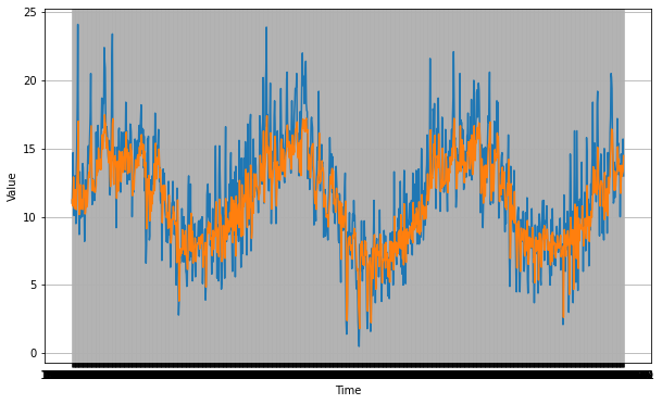
mse, mae = compute_metrics(series_valid, rnn_forecast)

print(f"mse: {mse:.2f}, mae: {mae:.2f} for forecast")

mse: 5.47, mae: 1.83 for forecast

To pass this assignment your forecast should achieve a MSE of 6 or less and a MAE of 2 or less.

• If your forecast didn’t achieve this threshold try re-training your model with a different architecture (you will need to re-run both create_uncompiled_model and create_model functions) or tweaking the optimizer’s parameters.

• If your forecast did achieve this threshold run the following cell to save the model in the SavedModel format which will be used for grading and after doing so, submit your assigment for grading.

• This environment includes a dummy SavedModel directory which contains a dummy model trained for one epoch. To replace this file with your actual model you need to run the next cell before submitting for grading.

# Save your model in the SavedModel format
model.save('saved_model/my_model')

# Compress the directory using tar
! tar -czvf saved_model.tar.gz saved_model/

INFO:tensorflow:Assets written to: saved_model/my_model/assets


INFO:tensorflow:Assets written to: saved_model/my_model/assets


saved_model/
saved_model/my_model/
saved_model/my_model/keras_metadata.pb
saved_model/my_model/variables/
saved_model/my_model/variables/variables.data-00000-of-00001
saved_model/my_model/variables/variables.index
saved_model/my_model/saved_model.pb
saved_model/my_model/assets/

Congratulations on finishing this week’s assignment!

You have successfully implemented a neural network capable of forecasting time series leveraging a combination of Tensorflow’s layers such as Convolutional and LSTMs! This resulted in a forecast that surpasses all the ones you did previously.

By finishing this assignment you have finished the specialization! Give yourself a pat on the back!!!

Please click here if you want to experiment with any of the non-graded code.

Important Note: Please only do this when you've already passed the assignment to avoid problems with the autograder.

1. On the notebook’s menu, click “View” > “Cell Toolbar” > “Edit Metadata”
2. Hit the “Edit Metadata” button next to the code cell which you want to lock/unlock
3. Set the attribute value for “editable” to:
   • “true” if you want to unlock it
   • “false” if you want to lock it
4. On the notebook’s menu, click “View” > “Cell Toolbar” > “None”

Here's a short demo of how to do the steps above: