Coursera

Week 2: Predicting time series

Welcome! In the previous assignment you got some exposure to working with time series data, but you didn’t use machine learning techniques for your forecasts. This week you will be using a deep neural network to create forecasts to see how this technique compares with the ones you already tried out. Once again all of the data is going to be generated.

Let’s get started!

NOTE: To prevent errors from the autograder, you are not allowed to edit or delete some of the cells in this notebook . Please only put your solutions in between the ### START CODE HERE and ### END CODE HERE code comments, and also refrain from adding any new cells. Once you have passed this assignment and want to experiment with any of the locked cells, you may follow the instructions at the bottom of this notebook.

import numpy as np
import tensorflow as tf
import matplotlib.pyplot as plt
from dataclasses import dataclass

Generating the data

The next cell includes a bunch of helper functions to generate and plot the time series:

def plot_series(time, series, format="-", start=0, end=None):
    plt.plot(time[start:end], series[start:end], format)
    plt.xlabel("Time")
    plt.ylabel("Value")
    plt.grid(False)

def trend(time, slope=0):
    return slope * time

def seasonal_pattern(season_time):
    """An arbitrary pattern"""
    return np.where(season_time < 0.1,
                    np.cos(season_time * 6 * np.pi), 
                    2 / np.exp(9 * season_time))

def seasonality(time, period, amplitude=1, phase=0):
    """Repeats the same pattern at each period"""
    season_time = ((time + phase) % period) / period
    return amplitude * seasonal_pattern(season_time)

def noise(time, noise_level=1, seed=None):
    rnd = np.random.RandomState(seed)
    return rnd.randn(len(time)) * noise_level

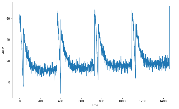
You will be generating time series data that greatly resembles the one from last week but with some differences.

Notice that this time all the generation is done within a function and global variables are saved within a dataclass. This is done to avoid using global scope as it was done in during the previous week.

If you haven’t used dataclasses before, they are just Python classes that provide a convenient syntax for storing data. You can read more about them in the docs.

def generate_time_series():
    # The time dimension or the x-coordinate of the time series
    time = np.arange(4 * 365 + 1, dtype="float32")

    # Initial series is just a straight line with a y-intercept
    y_intercept = 10
    slope = 0.005
    series = trend(time, slope) + y_intercept

    # Adding seasonality
    amplitude = 50
    series += seasonality(time, period=365, amplitude=amplitude)

    # Adding some noise
    noise_level = 3
    series += noise(time, noise_level, seed=51)
    
    return time, series


# Save all "global" variables within the G class (G stands for global)
@dataclass
class G:
    TIME, SERIES = generate_time_series()
    SPLIT_TIME = 1100
    WINDOW_SIZE = 20
    BATCH_SIZE = 32
    SHUFFLE_BUFFER_SIZE = 1000
    

# Plot the generated series
plt.figure(figsize=(10, 6))
plot_series(G.TIME, G.SERIES)
plt.show()

Splitting the data

Since you already coded the train_val_split function during last week’s assignment, this time it is provided for you:

def train_val_split(time, series, time_step=G.SPLIT_TIME):

    time_train = time[:time_step]
    series_train = series[:time_step]
    time_valid = time[time_step:]
    series_valid = series[time_step:]

    return time_train, series_train, time_valid, series_valid


# Split the dataset
time_train, series_train, time_valid, series_valid = train_val_split(G.TIME, G.SERIES)

Processing the data

As you saw on the lectures you can feed the data for training by creating a dataset with the appropiate processing steps such as windowing, flattening, batching and shuffling. To do so complete the windowed_dataset function below.

Notice that this function receives a series, window_size, batch_size and shuffle_buffer and the last three of these default to the “global” values defined earlier.

Be sure to check out the docs about TF Datasets if you need any help.

def windowed_dataset(series, window_size=G.WINDOW_SIZE, batch_size=G.BATCH_SIZE, shuffle_buffer=G.SHUFFLE_BUFFER_SIZE):
    
    ### START CODE HERE
    
    # Create dataset from the series
    dataset = tf.data.Dataset.from_tensor_slices(series)
    
    # Slice the dataset into the appropriate windows
    dataset = dataset.window(window_size + 1, shift=1, drop_remainder=True)
    
    # Flatten the dataset
    dataset = dataset.flat_map(lambda window: window.batch(window_size + 1))
    
    # Shuffle it
    dataset = dataset.shuffle(shuffle_buffer)
    
    # Split it into the features and labels
    dataset = dataset.map(lambda window: (window[:-1], window[-1]))
    
    # Batch it
    dataset = dataset.batch(batch_size).prefetch(1)
    
    ### END CODE HERE
    
    return dataset

To test your function you will be using a window_size of 1 which means that you will use each value to predict the next one. This for 5 elements since a batch_size of 5 is used and no shuffle since shuffle_buffer is set to 1.

Given this, the batch of features should be identical to the first 5 elements of the series_train and the batch of labels should be equal to elements 2 through 6 of the series_train.

# Test your function with windows size of 1 and no shuffling
test_dataset = windowed_dataset(series_train, window_size=1, batch_size=5, shuffle_buffer=1)

# Get the first batch of the test dataset
batch_of_features, batch_of_labels = next((iter(test_dataset)))

print(f"batch_of_features has type: {type(batch_of_features)}\n")
print(f"batch_of_labels has type: {type(batch_of_labels)}\n")
print(f"batch_of_features has shape: {batch_of_features.shape}\n")
print(f"batch_of_labels has shape: {batch_of_labels.shape}\n")
print(f"batch_of_features is equal to first five elements in the series: {np.allclose(batch_of_features.numpy().flatten(), series_train[:5])}\n")
print(f"batch_of_labels is equal to first five labels: {np.allclose(batch_of_labels.numpy(), series_train[1:6])}")

batch_of_features has type: <class 'tensorflow.python.framework.ops.EagerTensor'>

batch_of_labels has type: <class 'tensorflow.python.framework.ops.EagerTensor'>

batch_of_features has shape: (5, 1)

batch_of_labels has shape: (5,)

batch_of_features is equal to first five elements in the series: True

batch_of_labels is equal to first five labels: True

Expected Output:

batch_of_features has type: <class 'tensorflow.python.framework.ops.EagerTensor'>

batch_of_labels has type: <class 'tensorflow.python.framework.ops.EagerTensor'>

batch_of_features has shape: (5, 1)

batch_of_labels has shape: (5,)

batch_of_features is equal to first five elements in the series: True

batch_of_labels is equal to first five labels: True

Defining the model architecture

Now that you have a function that will process the data before it is fed into your neural network for training, it is time to define you layer architecture.

Complete the create_model function below. Notice that this function receives the window_size since this will be an important parameter for the first layer of your network.

Hint:

• You will only need Dense layers.
• Do not include Lambda layers. These are not required and are incompatible with the HDF5 format which will be used to save your model for grading.
• The training should be really quick so if you notice that each epoch is taking more than a few seconds, consider trying a different architecture.

def create_model(window_size=G.WINDOW_SIZE):

    ### START CODE HERE

    model = tf.keras.models.Sequential([ 
        tf.keras.layers.Dense(20, input_shape=[window_size], activation="relu"),
        tf.keras.layers.Dense(1)
    ]) 

    model.compile(loss="mse",
                  optimizer=tf.keras.optimizers.SGD(learning_rate=4e-6, momentum=0.9))
    
    ### END CODE HERE

    return model

# Apply the processing to the whole training series
dataset = windowed_dataset(series_train)

# Save an instance of the model
model = create_model()

# Train it
model.fit(dataset, epochs=100)

Epoch 1/100
34/34 [==============================] - 0s 1ms/step - loss: 432.0037
Epoch 2/100
34/34 [==============================] - 0s 772us/step - loss: 53.1036
Epoch 3/100
34/34 [==============================] - 0s 792us/step - loss: 43.9481
Epoch 4/100
34/34 [==============================] - 0s 722us/step - loss: 40.9097
Epoch 5/100
34/34 [==============================] - 0s 728us/step - loss: 38.6418
Epoch 6/100
34/34 [==============================] - 0s 818us/step - loss: 36.9632
Epoch 7/100
34/34 [==============================] - 0s 753us/step - loss: 35.4907
Epoch 8/100
34/34 [==============================] - 0s 835us/step - loss: 34.2192
Epoch 9/100
34/34 [==============================] - 0s 836us/step - loss: 33.2975
Epoch 10/100
34/34 [==============================] - 0s 840us/step - loss: 32.3960
Epoch 11/100
34/34 [==============================] - 0s 761us/step - loss: 31.8675
Epoch 12/100
34/34 [==============================] - 0s 725us/step - loss: 31.5957
Epoch 13/100
34/34 [==============================] - 0s 741us/step - loss: 31.0825
Epoch 14/100
34/34 [==============================] - 0s 779us/step - loss: 30.7385
Epoch 15/100
34/34 [==============================] - 0s 811us/step - loss: 30.6491
Epoch 16/100
34/34 [==============================] - 0s 771us/step - loss: 30.1697
Epoch 17/100
34/34 [==============================] - 0s 776us/step - loss: 30.0288
Epoch 18/100
34/34 [==============================] - 0s 719us/step - loss: 29.7878
Epoch 19/100
34/34 [==============================] - 0s 892us/step - loss: 29.7124
Epoch 20/100
34/34 [==============================] - 0s 826us/step - loss: 29.3897
Epoch 21/100
34/34 [==============================] - 0s 806us/step - loss: 29.1949
Epoch 22/100
34/34 [==============================] - 0s 802us/step - loss: 29.0864
Epoch 23/100
34/34 [==============================] - 0s 805us/step - loss: 28.9021
Epoch 24/100
34/34 [==============================] - 0s 792us/step - loss: 28.9995
Epoch 25/100
34/34 [==============================] - 0s 738us/step - loss: 28.7865
Epoch 26/100
34/34 [==============================] - 0s 789us/step - loss: 28.9492
Epoch 27/100
34/34 [==============================] - 0s 777us/step - loss: 28.4991
Epoch 28/100
34/34 [==============================] - 0s 852us/step - loss: 28.4334
Epoch 29/100
34/34 [==============================] - 0s 860us/step - loss: 28.1751
Epoch 30/100
34/34 [==============================] - 0s 863us/step - loss: 28.2371
Epoch 31/100
34/34 [==============================] - 0s 810us/step - loss: 28.1386
Epoch 32/100
34/34 [==============================] - 0s 749us/step - loss: 28.0834
Epoch 33/100
34/34 [==============================] - 0s 737us/step - loss: 27.8397
Epoch 34/100
34/34 [==============================] - 0s 717us/step - loss: 27.8064
Epoch 35/100
34/34 [==============================] - 0s 708us/step - loss: 27.7708
Epoch 36/100
34/34 [==============================] - 0s 754us/step - loss: 27.8721
Epoch 37/100
34/34 [==============================] - 0s 784us/step - loss: 27.7659
Epoch 38/100
34/34 [==============================] - 0s 711us/step - loss: 27.7820
Epoch 39/100
34/34 [==============================] - 0s 860us/step - loss: 27.4376
Epoch 40/100
34/34 [==============================] - 0s 838us/step - loss: 27.3057
Epoch 41/100
34/34 [==============================] - 0s 745us/step - loss: 27.2372
Epoch 42/100
34/34 [==============================] - 0s 814us/step - loss: 27.3107
Epoch 43/100
34/34 [==============================] - 0s 757us/step - loss: 27.1779
Epoch 44/100
34/34 [==============================] - 0s 842us/step - loss: 27.1299
Epoch 45/100
34/34 [==============================] - 0s 739us/step - loss: 27.1501
Epoch 46/100
34/34 [==============================] - 0s 796us/step - loss: 26.9611
Epoch 47/100
34/34 [==============================] - 0s 786us/step - loss: 27.0891
Epoch 48/100
34/34 [==============================] - 0s 720us/step - loss: 27.0048
Epoch 49/100
34/34 [==============================] - 0s 784us/step - loss: 26.8558
Epoch 50/100
34/34 [==============================] - 0s 722us/step - loss: 26.8591
Epoch 51/100
34/34 [==============================] - 0s 696us/step - loss: 26.8652
Epoch 52/100
34/34 [==============================] - 0s 1ms/step - loss: 26.8347
Epoch 53/100
34/34 [==============================] - 0s 789us/step - loss: 26.8090
Epoch 54/100
34/34 [==============================] - 0s 846us/step - loss: 26.8411
Epoch 55/100
34/34 [==============================] - 0s 814us/step - loss: 27.5792
Epoch 56/100
34/34 [==============================] - 0s 782us/step - loss: 26.6706
Epoch 57/100
34/34 [==============================] - 0s 817us/step - loss: 26.6676
Epoch 58/100
34/34 [==============================] - 0s 730us/step - loss: 26.5525
Epoch 59/100
34/34 [==============================] - 0s 791us/step - loss: 26.4576
Epoch 60/100
34/34 [==============================] - 0s 764us/step - loss: 26.5175
Epoch 61/100
34/34 [==============================] - 0s 765us/step - loss: 26.4752
Epoch 62/100
34/34 [==============================] - 0s 753us/step - loss: 26.5144
Epoch 63/100
34/34 [==============================] - 0s 835us/step - loss: 26.4172
Epoch 64/100
34/34 [==============================] - 0s 746us/step - loss: 26.4290
Epoch 65/100
34/34 [==============================] - 0s 821us/step - loss: 26.4485
Epoch 66/100
34/34 [==============================] - 0s 803us/step - loss: 26.3114
Epoch 67/100
34/34 [==============================] - 0s 791us/step - loss: 26.3403
Epoch 68/100
34/34 [==============================] - 0s 1ms/step - loss: 26.3533
Epoch 69/100
34/34 [==============================] - 0s 812us/step - loss: 26.5271
Epoch 70/100
34/34 [==============================] - 0s 794us/step - loss: 26.1934
Epoch 71/100
34/34 [==============================] - 0s 755us/step - loss: 26.4822
Epoch 72/100
34/34 [==============================] - 0s 725us/step - loss: 26.2346
Epoch 73/100
34/34 [==============================] - 0s 762us/step - loss: 26.1860
Epoch 74/100
34/34 [==============================] - 0s 729us/step - loss: 26.0801
Epoch 75/100
34/34 [==============================] - 0s 994us/step - loss: 26.0662
Epoch 76/100
34/34 [==============================] - 0s 766us/step - loss: 26.0646
Epoch 77/100
34/34 [==============================] - 0s 859us/step - loss: 26.0105
Epoch 78/100
34/34 [==============================] - 0s 814us/step - loss: 25.9541
Epoch 79/100
34/34 [==============================] - 0s 1ms/step - loss: 26.0285
Epoch 80/100
34/34 [==============================] - 0s 782us/step - loss: 25.9235
Epoch 81/100
34/34 [==============================] - 0s 755us/step - loss: 25.9328
Epoch 82/100
34/34 [==============================] - 0s 837us/step - loss: 26.0245
Epoch 83/100
34/34 [==============================] - 0s 971us/step - loss: 25.9526
Epoch 84/100
34/34 [==============================] - 0s 822us/step - loss: 26.0090
Epoch 85/100
34/34 [==============================] - 0s 892us/step - loss: 25.8742
Epoch 86/100
34/34 [==============================] - 0s 789us/step - loss: 25.8747
Epoch 87/100
34/34 [==============================] - 0s 735us/step - loss: 25.8353
Epoch 88/100
34/34 [==============================] - 0s 738us/step - loss: 26.0273
Epoch 89/100
34/34 [==============================] - 0s 726us/step - loss: 25.8941
Epoch 90/100
34/34 [==============================] - 0s 746us/step - loss: 25.7503
Epoch 91/100
34/34 [==============================] - 0s 738us/step - loss: 25.7409
Epoch 92/100
34/34 [==============================] - 0s 745us/step - loss: 25.6871
Epoch 93/100
34/34 [==============================] - 0s 727us/step - loss: 25.6798
Epoch 94/100
34/34 [==============================] - 0s 702us/step - loss: 25.6889
Epoch 95/100
34/34 [==============================] - 0s 1ms/step - loss: 25.5860
Epoch 96/100
34/34 [==============================] - 0s 830us/step - loss: 25.6218
Epoch 97/100
34/34 [==============================] - 0s 720us/step - loss: 25.5783
Epoch 98/100
34/34 [==============================] - 0s 737us/step - loss: 25.7704
Epoch 99/100
34/34 [==============================] - 0s 796us/step - loss: 25.6067
Epoch 100/100
34/34 [==============================] - 0s 800us/step - loss: 25.5268





<keras.callbacks.History at 0x7faa340524f0>

Evaluating the forecast

Now it is time to evaluate the performance of the forecast. For this you can use the compute_metrics function that you coded in the previous assignment:

def compute_metrics(true_series, forecast):
    
    mse = tf.keras.metrics.mean_squared_error(true_series, forecast).numpy()
    mae = tf.keras.metrics.mean_absolute_error(true_series, forecast).numpy()

    return mse, mae

At this point only the model that will perform the forecast is ready but you still need to compute the actual forecast.

For this, run the cell below which uses the generate_forecast function to compute the forecast. This function generates the next value given a set of the previous window_size points for every point in the validation set.

def generate_forecast(series=G.SERIES, split_time=G.SPLIT_TIME, window_size=G.WINDOW_SIZE):
    forecast = []
    for time in range(len(series) - window_size):
        forecast.append(model.predict(series[time:time + window_size][np.newaxis]))

    forecast = forecast[split_time-window_size:]
    results = np.array(forecast)[:, 0, 0]
    return results


# Save the forecast
dnn_forecast = generate_forecast()

# Plot it
plt.figure(figsize=(10, 6))
plot_series(time_valid, series_valid)
plot_series(time_valid, dnn_forecast)

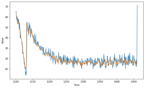
Expected Output:

A series similar to this one:

mse, mae = compute_metrics(series_valid, dnn_forecast)

print(f"mse: {mse:.2f}, mae: {mae:.2f} for forecast")

mse: 26.13, mae: 3.20 for forecast

To pass this assignment your forecast should achieve an MSE of 30 or less.

• If your forecast didn’t achieve this threshold try re-training your model with a different architecture or tweaking the optimizer’s parameters.

• If your forecast did achieve this threshold run the following cell to save your model in a HDF5 file file which will be used for grading and after doing so, submit your assigment for grading.

• Make sure you didn’t use Lambda layers in your model since these are incompatible with the HDF5 format which will be used to save your model for grading.

• This environment includes a dummy my_model.h5 file which is just a dummy model trained for one epoch. To replace this file with your actual model you need to run the next cell before submitting for grading.

# Save your model in HDF5 format
model.save('my_model.h5')

Congratulations on finishing this week’s assignment!

You have successfully implemented a neural network capable of forecasting time series while also learning how to leverage Tensorflow’s Dataset class to process time series data!

Keep it up!

Please click here if you want to experiment with any of the non-graded code.

Important Note: Please only do this when you've already passed the assignment to avoid problems with the autograder.

1. On the notebook’s menu, click “View” > “Cell Toolbar” > “Edit Metadata”
2. Hit the “Edit Metadata” button next to the code cell which you want to lock/unlock
3. Set the attribute value for “editable” to:
   • “true” if you want to unlock it
   • “false” if you want to lock it
4. On the notebook’s menu, click “View” > “Cell Toolbar” > “None”

Here's a short demo of how to do the steps above: