Coursera
Week 4: Handling Complex Images - Happy or Sad Dataset
In this assignment you will be using the happy or sad dataset, which contains 80 images of emoji-like faces, 40 happy and 40 sad.
Create a convolutional neural network that trains to 99.9% accuracy on these images, which cancels training upon hitting this training accuracy threshold.
# IMPORTANT: This will check your notebook's metadata for grading.
# Please do not continue the lab unless the output of this cell tells you to proceed.
!python add_metadata.py --filename C1W4_Assignment.ipynb
[32mGrader metadata detected! You can proceed with the lab![0m
NOTE: To prevent errors from the autograder, you are not allowed to edit or delete non-graded cells in this notebook . Please only put your solutions in between the ### START CODE HERE and ### END CODE HERE code comments, and also refrain from adding any new cells. Once you have passed this assignment and want to experiment with any of the non-graded code, you may follow the instructions at the bottom of this notebook.
# grader-required-cell

import matplotlib.pyplot as plt
import tensorflow as tf
import numpy as np
import os
Load and explore the data
Begin by taking a look at some images of the dataset.
Notice that all the images are contained within the ./data/ directory.
This directory contains two subdirectories happy/ and sad/ and each image is saved under the subdirectory related to the class it belongs to.
# grader-required-cell
from tensorflow.keras.preprocessing.image import load_img
base_dir = "./data/"
happy_dir = os.path.join(base_dir, "happy/")
sad_dir = os.path.join(base_dir, "sad/")
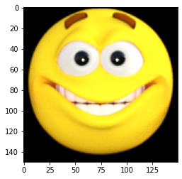
print("Sample happy image:")
plt.imshow(load_img(f"{os.path.join(happy_dir, os.listdir(happy_dir)[0])}"))
plt.show()
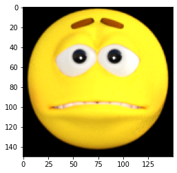
print("\nSample sad image:")
plt.imshow(load_img(f"{os.path.join(sad_dir, os.listdir(sad_dir)[0])}"))
plt.show()
Sample happy image:
Sample sad image:
It is cool to be able to see examples of the images to better understand the problem-space you are dealing with.
However there is still some relevant information that is missing such as the resolution of the image (although matplotlib renders the images in a grid providing a good idea of these values) and the maximum pixel value (this is important for normalizing these values). For this you can use Keras as shown in the next cell:
# grader-required-cell

from tensorflow.keras.preprocessing.image import img_to_array

# Load the first example of a happy face
sample_image  = load_img(f"{os.path.join(happy_dir, os.listdir(happy_dir)[0])}")

# Convert the image into its numpy array representation
sample_array = img_to_array(sample_image)

print(f"Each image has shape: {sample_array.shape}")

print(f"The maximum pixel value used is: {np.max(sample_array)}")
Each image has shape: (150, 150, 3)
The maximum pixel value used is: 255.0
Looks like the images have a resolution of 150x150. This is very important because this will be the input size of the first layer in your network.
The last dimension refers to each one of the 3 RGB channels that are used to represent colored images.
Defining the callback
Since you already have coded the callback responsible for stopping training (once a desired level of accuracy is reached) in the previous two assignments this time it is already provided so you can focus on the other steps:
# grader-required-cell

class myCallback(tf.keras.callbacks.Callback):
    def on_epoch_end(self, epoch, logs={}):
        if logs.get('accuracy') is not None and logs.get('accuracy') > 0.999:
            print("\nReached 99.9% accuracy so cancelling training!")
            self.model.stop_training = True
A quick note on callbacks:
So far you have used only the on_epoch_end callback but there are many more. For example you might want to check out the EarlyStopping callback, which allows you to save the best weights for your model.
Pre-processing the data
Keras provides great support for preprocessing image data. A lot can be accomplished by using the ImageDataGenerator class. Be sure to check out the docs if you get stuck in the next exercise. In particular you might want to pay attention to the rescale argument when instantiating the ImageDataGenerator and to the flow_from_directory method.
# grader-required-cell

from tensorflow.keras.preprocessing.image import ImageDataGenerator

# GRADED FUNCTION: image_generator
def image_generator():
    ### START CODE HERE

    # Instantiate the ImageDataGenerator class.
    # Remember to set the rescale argument.
    train_datagen = ImageDataGenerator(rescale=1/255)

    # Specify the method to load images from a directory and pass in the appropriate arguments:
    # - directory: should be a relative path to the directory containing the data
    # - targe_size: set this equal to the resolution of each image (excluding the color dimension)
    # - batch_size: number of images the generator yields when asked for a next batch. Set this to 10.
    # - class_mode: How the labels are represented. Should be one of "binary", "categorical" or "sparse".
    #               Pick the one that better suits here given that the labels are going to be 1D binary labels.
    train_generator = train_datagen.flow_from_directory(directory="./data/",
                                                        target_size=(150, 150),
                                                        batch_size=10,
                                                        class_mode="binary")
    ### END CODE HERE

    return train_generator
# grader-required-cell

# Save your generator in a variable
gen = image_generator()
Found 80 images belonging to 2 classes.
Expected Output:
Found 80 images belonging to 2 classes.
Creating and training your model
Finally, complete the train_happy_sad_model function below. This function should return your neural network.
Your model should achieve an accuracy of 99.9% or more before 15 epochs to pass this assignment.
Hints:
-
You can try any architecture for the network but keep in mind that the model will work best with 3 convolutional layers.
-
In case you need extra help you can check out some tips at the end of this notebook.
# grader-required-cell

from tensorflow.keras import optimizers, losses

# GRADED FUNCTION: train_happy_sad_model
def train_happy_sad_model(train_generator):

    # Instantiate the callback
    callbacks = myCallback()

    ### START CODE HERE

    # Define the model
    model = tf.keras.models.Sequential([
        tf.keras.layers.Conv2D(16, (3,3), activation='relu', input_shape=(150, 150, 3)),
        tf.keras.layers.MaxPooling2D(2, 2),
        # The second convolution
        tf.keras.layers.Conv2D(32, (3,3), activation='relu'),
        tf.keras.layers.MaxPooling2D(2,2),
        # The third convolution
        tf.keras.layers.Conv2D(64, (3,3), activation='relu'),
        tf.keras.layers.MaxPooling2D(2,2),
#     # The fourth convolution (You can uncomment the 4th and 5th conv layers later to see the effect)
#     tf.keras.layers.Conv2D(64, (3,3), activation='relu'),
#     tf.keras.layers.MaxPooling2D(2,2),
#     # The fifth convolution
#     tf.keras.layers.Conv2D(64, (3,3), activation='relu'),
#     tf.keras.layers.MaxPooling2D(2,2),
        # Flatten the results to feed into a DNN
        tf.keras.layers.Flatten(),
        # 512 neuron hidden layer
        tf.keras.layers.Dense(512, activation='relu'),
        # Only 1 output neuron. It will contain a value from 0-1 where 0 for 1 class ('horses') and 1 for the other ('humans')
        tf.keras.layers.Dense(1, activation='sigmoid')
    ])

    # Compile the model
    # Select a loss function compatible with the last layer of your network
    model.compile(loss="binary_crossentropy",
                  optimizer=optimizers.RMSprop(learning_rate=0.001),
                  metrics=['accuracy'])


    # Train the model
    # Your model should achieve the desired accuracy in less than 15 epochs.
    # You can hardcode up to 20 epochs in the function below but the callback should trigger before 15.
    history = model.fit(x=train_generator,
                        epochs=15,
                        callbacks=[callbacks]
                       )

    ### END CODE HERE
    return history
# grader-required-cell

hist = train_happy_sad_model(gen)
Epoch 1/15
8/8 [==============================] - 4s 429ms/step - loss: 3.4580 - accuracy: 0.6125
Epoch 2/15
8/8 [==============================] - 3s 401ms/step - loss: 0.5038 - accuracy: 0.7750
Epoch 3/15
8/8 [==============================] - 3s 414ms/step - loss: 0.1765 - accuracy: 0.9250
Epoch 4/15
8/8 [==============================] - 3s 399ms/step - loss: 0.1405 - accuracy: 0.9500
Epoch 5/15
8/8 [==============================] - 3s 371ms/step - loss: 0.1227 - accuracy: 0.9375
Epoch 6/15
8/8 [==============================] - 3s 401ms/step - loss: 0.2297 - accuracy: 0.8500
Epoch 7/15
8/8 [==============================] - 3s 401ms/step - loss: 0.0973 - accuracy: 0.9250
Epoch 8/15
8/8 [==============================] - ETA: 0s - loss: 0.0250 - accuracy: 1.0000
Reached 99.9% accuracy so cancelling training!
8/8 [==============================] - 3s 415ms/step - loss: 0.0250 - accuracy: 1.0000
If you see the message that was defined in the callback printed out after less than 15 epochs it means your callback worked as expected and training was successful. You can also double check by running the following cell:
# grader-required-cell

print(f"Your model reached the desired accuracy after {len(hist.epoch)} epochs")
Your model reached the desired accuracy after 8 epochs
If your callback didn’t stop training, one cause might be that you compiled your model using a metric other than accuracy (such as acc). Make sure you set the metric to accuracy. You can check by running the following cell:
if not "accuracy" in hist.model.metrics_names:
    print("Use 'accuracy' as metric when compiling your model.")
else:
    print("The metric was correctly defined.")
The metric was correctly defined.
Need more help?
Run the following cell to see some extra tips for the model’s architecture.
import base64

encoded_answer = "ClNvbWUgaGVscGZ1bCB0aXBzIGluIGNhc2UgeW91IGFyZSBzdHVjazoKCiAgICAtIEEgZ29vZCBmaXJzdCBsYXllciB3b3VsZCBiZSBhIENvbnYyRCBsYXllciB3aXRoIGFuIGlucHV0IHNoYXBlIHRoYXQgbWF0Y2hlcyAKICAgIHRoYXQgb2YgZXZlcnkgaW1hZ2UgaW4gdGhlIHRyYWluaW5nIHNldCAoaW5jbHVkaW5nIHRoZSBjb2xvciBkaW1lbnNpb24pCiAgICAKICAgIC0gVGhlIG1vZGVsIHdpbGwgd29yayBiZXN0IHdpdGggMyBjb252b2x1dGlvbmFsIGxheWVycwogICAgCiAgICAtIFRoZXJlIHNob3VsZCBiZSBhIEZsYXR0ZW4gbGF5ZXIgaW4gYmV0d2VlbiBjb252b2x1dGlvbmFsIGFuZCBkZW5zZSBsYXllcnMKICAgIAogICAgLSBUaGUgZmluYWwgbGF5ZXIgc2hvdWxkIGJlIGEgRGVuc2UgbGF5ZXIgd2l0aCB0aGUgbnVtYmVyIG9mIHVuaXRzIGFuZCAKICAgIGFjdGl2YXRpb24gZnVuY3Rpb24gdGhhdCBzdXBwb3J0cyBiaW5hcnkgY2xhc3NpZmljYXRpb24uCg=="
encoded_answer = encoded_answer.encode('ascii')
answer = base64.b64decode(encoded_answer)
answer = answer.decode('ascii')

print(answer)
Congratulations on finishing the last assignment of this course!
You have successfully implemented a CNN to assist you in the classification task for complex images. Nice job!
Keep it up!
Please click here if you want to experiment with any of the non-graded code.
Important Note: Please only do this when you've already passed the assignment to avoid problems with the autograder.
- On the notebook’s menu, click “View” > “Cell Toolbar” > “Edit Metadata”
- Hit the “Edit Metadata” button next to the code cell which you want to lock/unlock
- Set the attribute value for “editable” to:
- “true” if you want to unlock it
- “false” if you want to lock it
- On the notebook’s menu, click “View” > “Cell Toolbar” > “None”
Here's a short demo of how to do the steps above: