Coursera
Week 3: Variational Autoencoders on Anime Faces
For this exercise, you will train a Variational Autoencoder (VAE) using the anime faces dataset by MckInsey666.
You will train the model using the techniques discussed in class. At the end, you should save your model and download it from Colab so that it can be submitted to the autograder for grading.
Important: This colab notebook has read-only access so you won’t be able to save your changes. If you want to save your work periodically, please click File -> Save a Copy in Drive to create a copy in your account, then work from there.
Imports
# Install packages for compatibility with the autograder
!pip install tensorflow==2.8.0 --quiet
!pip install keras==2.8.0 --quiet
[31mERROR: pip's dependency resolver does not currently take into account all the packages that are installed. This behaviour is the source of the following dependency conflicts.
gcsfs 2023.6.0 requires fsspec==2023.6.0, but you have fsspec 2023.9.0 which is incompatible.
tensorflow-decision-forests 1.4.0 requires tensorflow~=2.12.0, but you have tensorflow 2.8.0 which is incompatible.
tensorflow-serving-api 2.12.1 requires tensorflow<3,>=2.12.0, but you have tensorflow 2.8.0 which is incompatible.
tensorflow-text 2.12.1 requires tensorflow<2.13,>=2.12.0; platform_machine != "arm64" or platform_system != "Darwin", but you have tensorflow 2.8.0 which is incompatible.[0m[31m
[0m
import tensorflow as tf
import tensorflow_datasets as tfds

import matplotlib.pyplot as plt
import numpy as np

import os
import zipfile
import urllib.request
import random
from IPython import display
/opt/conda/lib/python3.10/site-packages/scipy/__init__.py:146: UserWarning: A NumPy version >=1.16.5 and <1.23.0 is required for this version of SciPy (detected version 1.23.5
  warnings.warn(f"A NumPy version >={np_minversion} and <{np_maxversion}"
Parameters
# set a random seed
np.random.seed(51)

# parameters for building the model and training
BATCH_SIZE=2000
LATENT_DIM=512
IMAGE_SIZE=64
Download the Dataset
You will download the Anime Faces dataset and save it to a local directory.
# make the data directory
try:
  os.mkdir('/tmp/anime')
except OSError:
  pass

# download the zipped dataset to the data directory
data_url = "https://storage.googleapis.com/learning-datasets/Resources/anime-faces.zip"
data_file_name = "animefaces.zip"
download_dir = '/tmp/anime/'
urllib.request.urlretrieve(data_url, data_file_name)

# extract the zip file
zip_ref = zipfile.ZipFile(data_file_name, 'r')
zip_ref.extractall(download_dir)
zip_ref.close()
Prepare the Dataset
Next is preparing the data for training and validation. We’ve provided you some utilities below.
# Data Preparation Utilities

def get_dataset_slice_paths(image_dir):
  '''returns a list of paths to the image files'''
  image_file_list = os.listdir(image_dir)
  image_paths = [os.path.join(image_dir, fname) for fname in image_file_list]

  return image_paths


def map_image(image_filename):
  '''preprocesses the images'''
  img_raw = tf.io.read_file(image_filename)
  image = tf.image.decode_jpeg(img_raw)

  image = tf.cast(image, dtype=tf.float32)
  image = tf.image.resize(image, (IMAGE_SIZE, IMAGE_SIZE))
  image = image / 255.0
  image = tf.reshape(image, shape=(IMAGE_SIZE, IMAGE_SIZE, 3,))

  return image
You will use the functions above to generate the train and validation sets.
# get the list containing the image paths
paths = get_dataset_slice_paths("/tmp/anime/images/")

# shuffle the paths
random.shuffle(paths)

# split the paths list into to training (80%) and validation sets(20%).
paths_len = len(paths)
train_paths_len = int(paths_len * 0.8)

train_paths = paths[:train_paths_len]
val_paths = paths[train_paths_len:]

# load the training image paths into tensors, create batches and shuffle
training_dataset = tf.data.Dataset.from_tensor_slices((train_paths))
training_dataset = training_dataset.map(map_image)
training_dataset = training_dataset.shuffle(1000).batch(BATCH_SIZE)

# load the validation image paths into tensors and create batches
validation_dataset = tf.data.Dataset.from_tensor_slices((val_paths))
validation_dataset = validation_dataset.map(map_image)
validation_dataset = validation_dataset.batch(BATCH_SIZE)


print(f'number of batches in the training set: {len(training_dataset)}')
print(f'number of batches in the validation set: {len(validation_dataset)}')
number of batches in the training set: 26
number of batches in the validation set: 7
Display Utilities
We’ve also provided some utilities to help in visualizing the data.
def display_faces(dataset, size=9):
  '''Takes a sample from a dataset batch and plots it in a grid.'''
  dataset = dataset.unbatch().take(size)
  n_cols = 3
  n_rows = size//n_cols + 1
  plt.figure(figsize=(5, 5))
  i = 0
  for image in dataset:
    i += 1
    disp_img = np.reshape(image, (64,64,3))
    plt.subplot(n_rows, n_cols, i)
    plt.xticks([])
    plt.yticks([])
    plt.imshow(disp_img)


def display_one_row(disp_images, offset, shape=(28, 28)):
  '''Displays a row of images.'''
  for idx, image in enumerate(disp_images):
    plt.subplot(3, 10, offset + idx + 1)
    plt.xticks([])
    plt.yticks([])
    image = np.reshape(image, shape)
    plt.imshow(image)


def display_results(disp_input_images, disp_predicted):
  '''Displays input and predicted images.'''
  plt.figure(figsize=(15, 5))
  display_one_row(disp_input_images, 0, shape=(IMAGE_SIZE,IMAGE_SIZE,3))
  display_one_row(disp_predicted, 20, shape=(IMAGE_SIZE,IMAGE_SIZE,3))
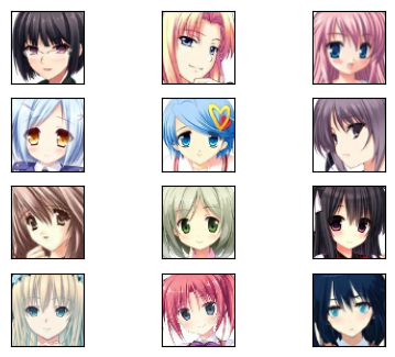
Let’s see some of the anime faces from the validation dataset.
display_faces(validation_dataset, size=12)
Build the Model
You will be building your VAE in the following sections. Recall that this will follow and encoder-decoder architecture and can be summarized by the figure below.
Sampling Class
You will start with the custom layer to provide the Gaussian noise input along with the mean (mu) and standard deviation (sigma) of the encoder’s output. Recall the equation to combine these:
$$z = \mu + e^{0.5\sigma} * \epsilon $$
where $\mu$ = mean, $\sigma$ = standard deviation, and $\epsilon$ = random sample
class Sampling(tf.keras.layers.Layer):
  def call(self, inputs):
    """Generates a random sample and combines with the encoder output

    Args:
      inputs -- output tensor from the encoder

    Returns:
      `inputs` tensors combined with a random sample
    """
    ### START CODE HERE ###
    mu, sigma = inputs
    batch = tf.shape(mu)[0]
    dim = tf.shape(mu)[1]
    epsilon = tf.keras.backend.random_normal(shape=(batch, dim))
    z = mu + tf.exp(0.5 * sigma) * epsilon
    ### END CODE HERE ###
    return  z
Encoder Layers
Next, please use the Functional API to stack the encoder layers and output mu, sigma and the shape of the features before flattening. We expect you to use 3 convolutional layers (instead of 2 in the ungraded lab) but feel free to revise as you see fit. Another hint is to use 1024 units in the Dense layer before you get mu and sigma (we used 20 for it in the ungraded lab).
Note: If you did Week 4 before Week 3, please do not use LeakyReLU activations yet for this particular assignment. The grader for Week 3 does not support LeakyReLU yet. This will be updated but for now, you can use relu and sigmoid just like in the ungraded lab.
def encoder_layers(inputs, latent_dim):
  """Defines the encoder's layers.
  Args:
    inputs -- batch from the dataset
    latent_dim -- dimensionality of the latent space

  Returns:
    mu -- learned mean
    sigma -- learned standard deviation
    batch_3.shape -- shape of the features before flattening
  """
  ### START CODE HERE ###
  x = tf.keras.layers.Conv2D(filters=16,
                             kernel_size=3,
                             strides=2,
                             padding="same",
                             name="encode_conv1")(inputs)
  x = tf.keras.layers.BatchNormalization()(x)
  x = tf.keras.layers.Conv2D(filters=32,
                             kernel_size=3,
                             strides=2,
                             padding="same",
                             name="encode_conv2")(x)
  x = tf.keras.layers.BatchNormalization()(x)
  x = tf.keras.layers.Conv2D(filters=64,
                             kernel_size=3,
                             strides=2,
                             padding="same",
                             name="encode_conv3")(x)
  batch_3 = tf.keras.layers.BatchNormalization()(x)

  x = tf.keras.layers.Flatten(name="encode_flatten")(batch_3)

  x = tf.keras.layers.Dense(1024, activation="relu", name="encode_dense")(x)
  x = tf.keras.layers.BatchNormalization()(x)

  mu = tf.keras.layers.Dense(latent_dim, name="latent_mu")(x)
  sigma = tf.keras.layers.Dense(latent_dim, name="latent_sigma")(x)
  ### END CODE HERE ###

  # revise `batch_3.shape` here if you opted not to use 3 Conv2D layers
  return mu, sigma, batch_3.shape
Encoder Model
You will feed the output from the above function to the Sampling layer you defined earlier. That will have the latent representations that can be fed to the decoder network later. Please complete the function below to build the encoder network with the Sampling layer.
def encoder_model(latent_dim, input_shape):
  """Defines the encoder model with the Sampling layer
  Args:
    latent_dim -- dimensionality of the latent space
    input_shape -- shape of the dataset batch

  Returns:
    model -- the encoder model
    conv_shape -- shape of the features before flattening
  """
  ### START CODE HERE ###
  inputs = tf.keras.layers.Input(shape=input_shape)
  mu, sigma, conv_shape = encoder_layers(inputs, latent_dim=latent_dim)
  z = Sampling()((mu, sigma))
  model = tf.keras.Model(inputs=inputs, outputs=[mu, sigma, z])
  ### END CODE HERE ###
  model.summary()
  return model, conv_shape
Decoder Layers
Next, you will define the decoder layers. This will expand the latent representations back to the original image dimensions. After training your VAE model, you can use this decoder model to generate new data by feeding random inputs.
def decoder_layers(inputs, conv_shape):
  """Defines the decoder layers.
  Args:
    inputs -- output of the encoder
    conv_shape -- shape of the features before flattening

  Returns:
    tensor containing the decoded output
  """
  ### START CODE HERE ###
  units = conv_shape[1] * conv_shape[2] * conv_shape[3]

  x = tf.keras.layers.Dense(units,
                            activation="relu",
                            name="decode_dense1")(inputs)
  x = tf.keras.layers.BatchNormalization()(x)

  x = tf.keras.layers.Reshape((conv_shape[1], conv_shape[2], conv_shape[3]),
                              name="decode_reshape")(x)

  x = tf.keras.layers.Conv2DTranspose(filters=64,
                                      kernel_size=3,
                                      strides=2,
                                      padding="same",
                                      activation="relu",
                                      name="decode_conv2d_2")(x)
  x = tf.keras.layers.BatchNormalization()(x)

  x = tf.keras.layers.Conv2DTranspose(filters=32,
                                      kernel_size=3,
                                      strides=2,
                                      padding="same",
                                      activation="relu",
                                      name="decode_conv2d_3")(x)
  x = tf.keras.layers.BatchNormalization()(x)

  x = tf.keras.layers.Conv2DTranspose(filters=16,
                                      kernel_size=3,
                                      strides=2,
                                      padding="same",
                                      activation="relu",
                                      name="decode_conv2d_4")(x)
  x = tf.keras.layers.BatchNormalization()(x)

  x = tf.keras.layers.Conv2DTranspose(filters=3,
                                      kernel_size=3,
                                      strides=1,
                                      padding="same",
                                      activation="sigmoid",
                                      name="decode_final")(x)
  ### END CODE HERE ###
  return x
Decoder Model
Please complete the function below to output the decoder model.
def decoder_model(latent_dim, conv_shape):
  """Defines the decoder model.
  Args:
    latent_dim -- dimensionality of the latent space
    conv_shape -- shape of the features before flattening

  Returns:
    model -- the decoder model
  """
  ### START CODE HERE ###
  inputs = tf.keras.layers.Input(shape=(latent_dim,))
  outputs = decoder_layers(inputs, conv_shape)
  model = tf.keras.Model(inputs=inputs, outputs=outputs)
  ### END CODE HERE ###
  model.summary()
  return model
Kullback–Leibler Divergence
Next, you will define the function to compute the Kullback–Leibler Divergence loss. This will be used to improve the generative capability of the model. This code is already given.
def kl_reconstruction_loss(mu, sigma):
  """ Computes the Kullback-Leibler Divergence (KLD)
  Args:
    mu -- mean
    sigma -- standard deviation

  Returns:
    KLD loss
  """
  kl_loss = 1 + sigma - tf.square(mu) - tf.math.exp(sigma)
  return tf.reduce_mean(kl_loss) * -0.5
Putting it all together
Please define the whole VAE model. Remember to use model.add_loss() to add the KL reconstruction loss. This will be accessed and added to the loss later in the training loop.
def vae_model(encoder, decoder, input_shape):
  """Defines the VAE model
  Args:
    encoder -- the encoder model
    decoder -- the decoder model
    input_shape -- shape of the dataset batch

  Returns:
    the complete VAE model
  """
  ### START CODE HERE ###
  inputs = tf.keras.layers.Input(shape=input_shape)

  mu, sigma, z = encoder(inputs)

  reconstructed = decoder(z)

  model = tf.keras.Model(inputs=inputs, outputs=reconstructed)

  loss = kl_reconstruction_loss(mu, sigma)

  model.add_loss(loss)

  ### END CODE HERE ###
  return model
Next, please define a helper function to return the encoder, decoder, and vae models you just defined.
def get_models(input_shape, latent_dim):
  """Returns the encoder, decoder, and vae models"""
  ### START CODE HERE ###
  encoder, conv_shape = encoder_model(
      latent_dim=latent_dim,
      input_shape=input_shape
  )

  decoder = decoder_model(
      latent_dim=latent_dim,
      conv_shape=conv_shape
  )

  vae = vae_model(encoder, decoder, input_shape=input_shape)

  ### END CODE HERE ###
  return encoder, decoder, vae
Let’s use the function above to get the models we need in the training loop.
encoder, decoder, vae = get_models(input_shape=(64,64,3,), latent_dim=LATENT_DIM)
Model: "model"
__________________________________________________________________________________________________
 Layer (type)                   Output Shape         Param #     Connected to
==================================================================================================
 input_1 (InputLayer)           [(None, 64, 64, 3)]  0           []

 encode_conv1 (Conv2D)          (None, 32, 32, 16)   448         ['input_1[0][0]']

 batch_normalization (BatchNorm  (None, 32, 32, 16)  64          ['encode_conv1[0][0]']
 alization)

 encode_conv2 (Conv2D)          (None, 16, 16, 32)   4640        ['batch_normalization[0][0]']

 batch_normalization_1 (BatchNo  (None, 16, 16, 32)  128         ['encode_conv2[0][0]']
 rmalization)

 encode_conv3 (Conv2D)          (None, 8, 8, 64)     18496       ['batch_normalization_1[0][0]']

 batch_normalization_2 (BatchNo  (None, 8, 8, 64)    256         ['encode_conv3[0][0]']
 rmalization)

 encode_flatten (Flatten)       (None, 4096)         0           ['batch_normalization_2[0][0]']

 encode_dense (Dense)           (None, 1024)         4195328     ['encode_flatten[0][0]']

 batch_normalization_3 (BatchNo  (None, 1024)        4096        ['encode_dense[0][0]']
 rmalization)

 latent_mu (Dense)              (None, 512)          524800      ['batch_normalization_3[0][0]']

 latent_sigma (Dense)           (None, 512)          524800      ['batch_normalization_3[0][0]']

 sampling (Sampling)            (None, 512)          0           ['latent_mu[0][0]',
                                                                  'latent_sigma[0][0]']

==================================================================================================
Total params: 5,273,056
Trainable params: 5,270,784
Non-trainable params: 2,272
__________________________________________________________________________________________________
Model: "model_1"
_________________________________________________________________
 Layer (type)                Output Shape              Param #
=================================================================
 input_2 (InputLayer)        [(None, 512)]             0

 decode_dense1 (Dense)       (None, 4096)              2101248

 batch_normalization_4 (Batc  (None, 4096)             16384
 hNormalization)

 decode_reshape (Reshape)    (None, 8, 8, 64)          0

 decode_conv2d_2 (Conv2DTran  (None, 16, 16, 64)       36928
 spose)

 batch_normalization_5 (Batc  (None, 16, 16, 64)       256
 hNormalization)

 decode_conv2d_3 (Conv2DTran  (None, 32, 32, 32)       18464
 spose)

 batch_normalization_6 (Batc  (None, 32, 32, 32)       128
 hNormalization)

 decode_conv2d_4 (Conv2DTran  (None, 64, 64, 16)       4624
 spose)

 batch_normalization_7 (Batc  (None, 64, 64, 16)       64
 hNormalization)

 decode_final (Conv2DTranspo  (None, 64, 64, 3)        435
 se)

=================================================================
Total params: 2,178,531
Trainable params: 2,170,115
Non-trainable params: 8,416
_________________________________________________________________
Train the Model
You will now configure the model for training. We defined some losses, the optimizer, and the loss metric below but you can experiment with others if you like.
optimizer = tf.keras.optimizers.Adam(learning_rate=0.002)
loss_metric = tf.keras.metrics.Mean()
mse_loss = tf.keras.losses.MeanSquaredError()
bce_loss = tf.keras.losses.BinaryCrossentropy()
You will generate 16 images in a 4x4 grid to show progress of image generation. We’ve defined a utility function for that below.
def generate_and_save_images(model, epoch, step, test_input):
  """Helper function to plot our 16 images

  Args:

  model -- the decoder model
  epoch -- current epoch number during training
  step -- current step number during training
  test_input -- random tensor with shape (16, LATENT_DIM)
  """
  predictions = model.predict(test_input)

  fig = plt.figure(figsize=(4,4))

  for i in range(predictions.shape[0]):
      plt.subplot(4, 4, i+1)
      img = predictions[i, :, :, :] * 255
      img = img.astype('int32')
      plt.imshow(img)
      plt.axis('off')

  # tight_layout minimizes the overlap between 2 sub-plots
  fig.suptitle("epoch: {}, step: {}".format(epoch, step))
  plt.savefig('image_at_epoch_{:04d}_step{:04d}.png'.format(epoch, step))
  plt.show()
You can now start the training loop. You are asked to select the number of epochs and to complete the subection on updating the weights. The general steps are:
- feed a training batch to the VAE model
- compute the reconstruction loss (hint: use the mse_loss defined above instead of
bce_lossin the ungraded lab, then multiply by the flattened dimensions of the image (i.e. 64 x 64 x 3) - add the KLD regularization loss to the total loss (you can access the
lossesproperty of thevaemodel) - get the gradients
- use the optimizer to update the weights
When training your VAE, you might notice that there’s not a lot of variation in the faces. But don’t let that deter you! We’ll test based on how well it does in reconstructing the original faces, and not how well it does in creating new faces.
The training will also take a long time (more than 30 minutes) and that is to be expected. If you used the mean loss metric suggested above, train the model until that is down to around 320 before submitting.
# Training loop. Display generated images each epoch

### START CODE HERE ###
epochs = 100
### END CODE HERE ###

random_vector_for_generation = tf.random.normal(shape=[16, LATENT_DIM])
generate_and_save_images(decoder, 0, 0, random_vector_for_generation)

for epoch in range(epochs):
  print('Start of epoch %d' % (epoch,))

  # Iterate over the batches of the dataset.
  for step, x_batch_train in enumerate(training_dataset):
    with tf.GradientTape() as tape:
      ### START CODE HERE ###
      reconstructed = vae(x_batch_train)
      # Compute reconstruction loss
      flattened_inputs = tf.reshape(x_batch_train, shape=[-1])
      flattened_outputs = tf.reshape(reconstructed, shape=[-1])
      loss = mse_loss(flattened_inputs, flattened_outputs) * 64 * 64 * 3

      loss += sum(vae.losses)

    grads = tape.gradient(loss, vae.trainable_weights)
    optimizer.apply_gradients(zip(grads, vae.trainable_weights))
    ### END CODE HERE

    loss_metric(loss)

    loss_number = loss_metric.result().numpy()

    if step % 10 == 0:
#       display.clear_output(wait=False)
#       generate_and_save_images(decoder, epoch, step, random_vector_for_generation)
      print('Epoch: %s step: %s mean loss = %s' % (epoch, step, loss_metric.result().numpy()))

    # Early stopping
    if loss_number <= 300:
        break
Start of epoch 0
Epoch: 0 step: 0 mean loss = 1160.88
Epoch: 0 step: 10 mean loss = 906.783
Epoch: 0 step: 20 mean loss = 836.1077
Start of epoch 1
Epoch: 1 step: 0 mean loss = 803.84924
Epoch: 1 step: 10 mean loss = 758.6369
Epoch: 1 step: 20 mean loss = 722.31323
Start of epoch 2
Epoch: 2 step: 0 mean loss = 705.44684
Epoch: 2 step: 10 mean loss = 680.02686
Epoch: 2 step: 20 mean loss = 657.5172
Start of epoch 3
Epoch: 3 step: 0 mean loss = 644.83655
Epoch: 3 step: 10 mean loss = 626.3797
Epoch: 3 step: 20 mean loss = 609.65204
Start of epoch 4
Epoch: 4 step: 0 mean loss = 600.2716
Epoch: 4 step: 10 mean loss = 585.3218
Epoch: 4 step: 20 mean loss = 572.1631
Start of epoch 5
Epoch: 5 step: 0 mean loss = 564.6443
Epoch: 5 step: 10 mean loss = 552.74554
Epoch: 5 step: 20 mean loss = 542.0102
Start of epoch 6
Epoch: 6 step: 0 mean loss = 535.7973
Epoch: 6 step: 10 mean loss = 526.0139
Epoch: 6 step: 20 mean loss = 516.8958
Start of epoch 7
Epoch: 7 step: 0 mean loss = 511.58295
Epoch: 7 step: 10 mean loss = 502.7391
Epoch: 7 step: 20 mean loss = 494.33972
Start of epoch 8
Epoch: 8 step: 0 mean loss = 489.35898
Epoch: 8 step: 10 mean loss = 481.2276
Epoch: 8 step: 20 mean loss = 473.11978
Start of epoch 9
Epoch: 9 step: 0 mean loss = 469.3356
Epoch: 9 step: 10 mean loss = 463.4369
Epoch: 9 step: 20 mean loss = 456.85257
Start of epoch 10
Epoch: 10 step: 0 mean loss = 452.8546
Epoch: 10 step: 10 mean loss = 446.2781
Epoch: 10 step: 20 mean loss = 439.90564
Start of epoch 11
Epoch: 11 step: 0 mean loss = 436.39804
Epoch: 11 step: 10 mean loss = 431.05084
Epoch: 11 step: 20 mean loss = 425.5385
Start of epoch 12
Epoch: 12 step: 0 mean loss = 422.2764
Epoch: 12 step: 10 mean loss = 417.32455
Epoch: 12 step: 20 mean loss = 412.8162
Start of epoch 13
Epoch: 13 step: 0 mean loss = 409.99332
Epoch: 13 step: 10 mean loss = 405.2939
Epoch: 13 step: 20 mean loss = 400.70782
Start of epoch 14
Epoch: 14 step: 0 mean loss = 398.15027
Epoch: 14 step: 10 mean loss = 394.52597
Epoch: 14 step: 20 mean loss = 390.5492
Start of epoch 15
Epoch: 15 step: 0 mean loss = 388.15375
Epoch: 15 step: 10 mean loss = 384.22186
Epoch: 15 step: 20 mean loss = 380.37808
Start of epoch 16
Epoch: 16 step: 0 mean loss = 378.30905
Epoch: 16 step: 10 mean loss = 375.13315
Epoch: 16 step: 20 mean loss = 371.755
Start of epoch 17
Epoch: 17 step: 0 mean loss = 369.72162
Epoch: 17 step: 10 mean loss = 366.40274
Epoch: 17 step: 20 mean loss = 363.39584
Start of epoch 18
Epoch: 18 step: 0 mean loss = 361.6563
Epoch: 18 step: 10 mean loss = 358.66382
Epoch: 18 step: 20 mean loss = 355.68622
Start of epoch 19
Epoch: 19 step: 0 mean loss = 353.92212
Epoch: 19 step: 10 mean loss = 351.40204
Epoch: 19 step: 20 mean loss = 348.9111
Start of epoch 20
Epoch: 20 step: 0 mean loss = 347.35434
Epoch: 20 step: 10 mean loss = 344.74237
Epoch: 20 step: 20 mean loss = 342.15314
Start of epoch 21
Epoch: 21 step: 0 mean loss = 340.6209
Epoch: 21 step: 10 mean loss = 338.27643
Epoch: 21 step: 20 mean loss = 335.89386
Start of epoch 22
Epoch: 22 step: 0 mean loss = 334.4597
Epoch: 22 step: 10 mean loss = 332.12494
Epoch: 22 step: 20 mean loss = 330.08536
Start of epoch 23
Epoch: 23 step: 0 mean loss = 328.81186
Epoch: 23 step: 10 mean loss = 326.66525
Epoch: 23 step: 20 mean loss = 324.55844
Start of epoch 24
Epoch: 24 step: 0 mean loss = 323.9527
Epoch: 24 step: 10 mean loss = 322.3849
Epoch: 24 step: 20 mean loss = 320.5634
Start of epoch 25
Epoch: 25 step: 0 mean loss = 319.43362
Epoch: 25 step: 10 mean loss = 317.5376
Epoch: 25 step: 20 mean loss = 315.74554
Start of epoch 26
Epoch: 26 step: 0 mean loss = 314.658
Epoch: 26 step: 10 mean loss = 312.83978
Epoch: 26 step: 20 mean loss = 311.0417
Start of epoch 27
Epoch: 27 step: 0 mean loss = 310.01062
Epoch: 27 step: 10 mean loss = 308.2818
Epoch: 27 step: 20 mean loss = 306.56155
Start of epoch 28
Epoch: 28 step: 0 mean loss = 305.58487
Epoch: 28 step: 10 mean loss = 303.9699
Epoch: 28 step: 20 mean loss = 302.35223
Start of epoch 29
Epoch: 29 step: 0 mean loss = 301.40387
Epoch: 29 step: 10 mean loss = 299.9031
Start of epoch 30
Epoch: 30 step: 0 mean loss = 299.752
Start of epoch 31
Epoch: 31 step: 0 mean loss = 299.60388
Start of epoch 32
Epoch: 32 step: 0 mean loss = 299.45676
Start of epoch 33
Epoch: 33 step: 0 mean loss = 299.31332
Start of epoch 34
Epoch: 34 step: 0 mean loss = 299.16672
Start of epoch 35
Epoch: 35 step: 0 mean loss = 299.01428
Start of epoch 36
Epoch: 36 step: 0 mean loss = 298.8603
Start of epoch 37
Epoch: 37 step: 0 mean loss = 298.7047
Start of epoch 38
Epoch: 38 step: 0 mean loss = 298.55078
Start of epoch 39
Epoch: 39 step: 0 mean loss = 298.3991
Start of epoch 40
Epoch: 40 step: 0 mean loss = 298.24875
Start of epoch 41
Epoch: 41 step: 0 mean loss = 298.09567
Start of epoch 42
Epoch: 42 step: 0 mean loss = 297.93967
Start of epoch 43
Epoch: 43 step: 0 mean loss = 297.7848
Start of epoch 44
Epoch: 44 step: 0 mean loss = 297.62918
Start of epoch 45
Epoch: 45 step: 0 mean loss = 297.47342
Start of epoch 46
Epoch: 46 step: 0 mean loss = 297.31808
Start of epoch 47
Epoch: 47 step: 0 mean loss = 297.16357
Start of epoch 48
Epoch: 48 step: 0 mean loss = 297.00967
Start of epoch 49
Epoch: 49 step: 0 mean loss = 296.85483
Start of epoch 50
Epoch: 50 step: 0 mean loss = 296.69943
Start of epoch 51
Epoch: 51 step: 0 mean loss = 296.5435
Start of epoch 52
Epoch: 52 step: 0 mean loss = 296.38577
Start of epoch 53
Epoch: 53 step: 0 mean loss = 296.22906
Start of epoch 54
Epoch: 54 step: 0 mean loss = 296.073
Start of epoch 55
Epoch: 55 step: 0 mean loss = 295.91647
Start of epoch 56
Epoch: 56 step: 0 mean loss = 295.76086
Start of epoch 57
Epoch: 57 step: 0 mean loss = 295.60394
Start of epoch 58
Epoch: 58 step: 0 mean loss = 295.44916
Start of epoch 59
Epoch: 59 step: 0 mean loss = 295.29477
Start of epoch 60
Epoch: 60 step: 0 mean loss = 295.1379
Start of epoch 61
Epoch: 61 step: 0 mean loss = 294.98053
Start of epoch 62
Epoch: 62 step: 0 mean loss = 294.82486
Start of epoch 63
Epoch: 63 step: 0 mean loss = 294.669
Start of epoch 64
Epoch: 64 step: 0 mean loss = 294.51505
Start of epoch 65
Epoch: 65 step: 0 mean loss = 294.3623
Start of epoch 66
Epoch: 66 step: 0 mean loss = 294.21234
Start of epoch 67
Epoch: 67 step: 0 mean loss = 294.06833
Start of epoch 68
Epoch: 68 step: 0 mean loss = 293.93198
Start of epoch 69
Epoch: 69 step: 0 mean loss = 293.7921
Start of epoch 70
Epoch: 70 step: 0 mean loss = 293.65143
Start of epoch 71
Epoch: 71 step: 0 mean loss = 293.50934
Start of epoch 72
Epoch: 72 step: 0 mean loss = 293.36017
Start of epoch 73
Epoch: 73 step: 0 mean loss = 293.2165
Start of epoch 74
Epoch: 74 step: 0 mean loss = 293.06958
Start of epoch 75
Epoch: 75 step: 0 mean loss = 292.92566
Start of epoch 76
Epoch: 76 step: 0 mean loss = 292.78027
Start of epoch 77
Epoch: 77 step: 0 mean loss = 292.63544
Start of epoch 78
Epoch: 78 step: 0 mean loss = 292.49265
Start of epoch 79
Epoch: 79 step: 0 mean loss = 292.35254
Start of epoch 80
Epoch: 80 step: 0 mean loss = 292.21353
Start of epoch 81
Epoch: 81 step: 0 mean loss = 292.07437
Start of epoch 82
Epoch: 82 step: 0 mean loss = 291.93002
Start of epoch 83
Epoch: 83 step: 0 mean loss = 291.78256
Start of epoch 84
Epoch: 84 step: 0 mean loss = 291.63333
Start of epoch 85
Epoch: 85 step: 0 mean loss = 291.4844
Start of epoch 86
Epoch: 86 step: 0 mean loss = 291.33752
Start of epoch 87
Epoch: 87 step: 0 mean loss = 291.19507
Start of epoch 88
Epoch: 88 step: 0 mean loss = 291.05194
Start of epoch 89
Epoch: 89 step: 0 mean loss = 290.90765
Start of epoch 90
Epoch: 90 step: 0 mean loss = 290.76028
Start of epoch 91
Epoch: 91 step: 0 mean loss = 290.61295
Start of epoch 92
Epoch: 92 step: 0 mean loss = 290.46408
Start of epoch 93
Epoch: 93 step: 0 mean loss = 290.31638
Start of epoch 94
Epoch: 94 step: 0 mean loss = 290.1671
Start of epoch 95
Epoch: 95 step: 0 mean loss = 290.01898
Start of epoch 96
Epoch: 96 step: 0 mean loss = 289.8722
Start of epoch 97
Epoch: 97 step: 0 mean loss = 289.7257
Start of epoch 98
Epoch: 98 step: 0 mean loss = 289.58078
Start of epoch 99
Epoch: 99 step: 0 mean loss = 289.43546
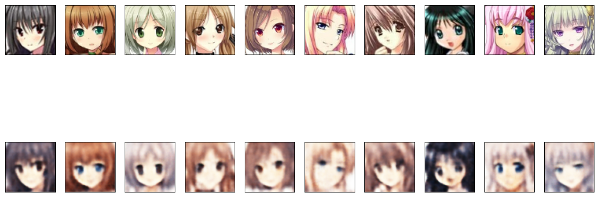
Plot Reconstructed Images
As mentioned, your model will be graded on how well it is able to reconstruct images (not generate new ones). You can get a glimpse of how it is doing with the code block below. It feeds in a batch from the test set and plots a row of input (top) and output (bottom) images. Don’t worry if the outputs are a blurry. It will look something like below:
test_dataset = validation_dataset.take(1)
output_samples = []

for input_image in tfds.as_numpy(test_dataset):
      output_samples = input_image

idxs = np.random.choice(64, size=10)

vae_predicted = vae.predict(test_dataset)
display_results(output_samples[idxs], vae_predicted[idxs])
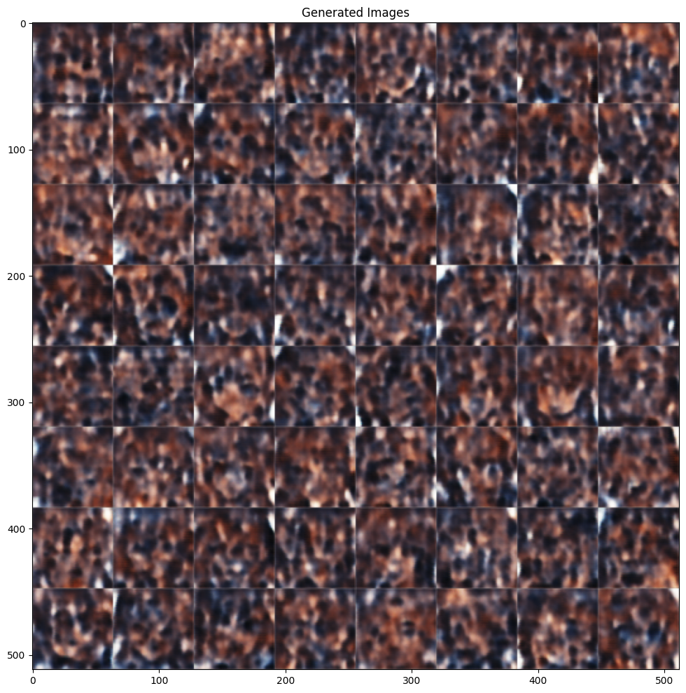
Plot Generated Images
Using the default parameters, it can take a long time to train your model well enough to generate good fake anime faces. In case you decide to experiment, we provided the code block below to display an 8x8 gallery of fake data generated from your model. Here is a sample gallery generated after 50 epochs.
def plot_images(rows, cols, images, title):
    '''Displays images in a grid.'''
    grid = np.zeros(shape=(rows*64, cols*64, 3))
    for row in range(rows):
        for col in range(cols):
            grid[row*64:(row+1)*64, col*64:(col+1)*64, :] = images[row*cols + col]

    plt.figure(figsize=(12,12))
    plt.imshow(grid)
    plt.title(title)
    plt.show()

# initialize random inputs
test_vector_for_generation = tf.random.normal(shape=[64, LATENT_DIM])

# get predictions from the decoder model
predictions= decoder.predict(test_vector_for_generation)

# plot the predictions
plot_images(8,8,predictions,'Generated Images')
Save the Model
Once your satisfied with the results, please save and download the model. Afterwards, please go back to the Coursera submission portal to upload your h5 file to the autograder.
vae.save("anime.h5")