Coursera
Ungraded Lab: Convolutional Autoencoders
In this lab, you will use convolution layers to build your autoencoder. This usually leads to better results than dense networks and you will see it in action with the Fashion MNIST dataset.
Imports
try:
  # %tensorflow_version only exists in Colab.
  %tensorflow_version 2.x
except Exception:
  pass

import tensorflow as tf
import tensorflow_datasets as tfds

import numpy as np
import matplotlib.pyplot as plt
Colab only includes TensorFlow 2.x; %tensorflow_version has no effect.
Prepare the Dataset
As before, you will load the train and test sets from TFDS. Notice that we don’t flatten the image this time. That’s because we will be using convolutional layers later that can deal with 2D images.
def map_image(image, label):
  '''Normalizes the image. Returns image as input and label.'''
  image = tf.cast(image, dtype=tf.float32)
  image = image / 255.0

  return image, image
BATCH_SIZE = 128
SHUFFLE_BUFFER_SIZE = 1024

train_dataset = tfds.load('fashion_mnist', as_supervised=True, split="train")
train_dataset = train_dataset.map(map_image)
train_dataset = train_dataset.shuffle(SHUFFLE_BUFFER_SIZE).batch(BATCH_SIZE).repeat()

test_dataset = tfds.load('fashion_mnist', as_supervised=True, split="test")
test_dataset = test_dataset.map(map_image)
test_dataset = test_dataset.batch(BATCH_SIZE).repeat()
Downloading and preparing dataset 29.45 MiB (download: 29.45 MiB, generated: 36.42 MiB, total: 65.87 MiB) to /root/tensorflow_datasets/fashion_mnist/3.0.1...


Dl Completed...: 0 url [00:00, ? url/s]


Dl Size...: 0 MiB [00:00, ? MiB/s]


Extraction completed...: 0 file [00:00, ? file/s]


Generating splits...:   0%|          | 0/2 [00:00<?, ? splits/s]


Generating train examples...:   0%|          | 0/60000 [00:00<?, ? examples/s]


Shuffling /root/tensorflow_datasets/fashion_mnist/3.0.1.incompleteHC5D4L/fashion_mnist-train.tfrecord*...:   0…


Generating test examples...:   0%|          | 0/10000 [00:00<?, ? examples/s]


Shuffling /root/tensorflow_datasets/fashion_mnist/3.0.1.incompleteHC5D4L/fashion_mnist-test.tfrecord*...:   0%…


Dataset fashion_mnist downloaded and prepared to /root/tensorflow_datasets/fashion_mnist/3.0.1. Subsequent calls will reuse this data.
Define the Model
As mentioned, you will use convolutional layers to build the model. This is composed of three main parts: encoder, bottleneck, and decoder. You will follow the configuration shown in the image below.
The encoder, just like in previous labs, will contract with each additional layer. The features are generated with the Conv2D layers while the max pooling layers reduce the dimensionality.
def encoder(inputs):
  '''Defines the encoder with two Conv2D and max pooling layers.'''
  conv_1 = tf.keras.layers.Conv2D(filters=64, kernel_size=(3,3), activation='relu', padding='same')(inputs)
  max_pool_1 = tf.keras.layers.MaxPooling2D(pool_size=(2,2))(conv_1)

  conv_2 = tf.keras.layers.Conv2D(filters=128, kernel_size=(3,3), activation='relu', padding='same')(max_pool_1)
  max_pool_2 = tf.keras.layers.MaxPooling2D(pool_size=(2,2))(conv_2)

  return max_pool_2
A bottleneck layer is used to get more features but without further reducing the dimension afterwards. Another layer is inserted here for visualizing the encoder output.
def bottle_neck(inputs):
  '''Defines the bottleneck.'''
  bottle_neck = tf.keras.layers.Conv2D(filters=256, kernel_size=(3,3), activation='relu', padding='same')(inputs)
  encoder_visualization = tf.keras.layers.Conv2D(filters=1, kernel_size=(3,3), activation='sigmoid', padding='same')(bottle_neck)

  return bottle_neck, encoder_visualization
The decoder will upsample the bottleneck output back to the original image size.
def decoder(inputs):
  '''Defines the decoder path to upsample back to the original image size.'''
  conv_1 = tf.keras.layers.Conv2D(filters=128, kernel_size=(3,3), activation='relu', padding='same')(inputs)
  up_sample_1 = tf.keras.layers.UpSampling2D(size=(2,2))(conv_1)

  conv_2 = tf.keras.layers.Conv2D(filters=64, kernel_size=(3,3), activation='relu', padding='same')(up_sample_1)
  up_sample_2 = tf.keras.layers.UpSampling2D(size=(2,2))(conv_2)

  conv_3 = tf.keras.layers.Conv2D(filters=1, kernel_size=(3,3), activation='sigmoid', padding='same')(up_sample_2)

  return conv_3
You can now build the full autoencoder using the functions above.
def convolutional_auto_encoder():
  '''Builds the entire autoencoder model.'''
  inputs = tf.keras.layers.Input(shape=(28, 28, 1,))
  encoder_output = encoder(inputs)
  bottleneck_output, encoder_visualization = bottle_neck(encoder_output)
  decoder_output = decoder(bottleneck_output)

  model = tf.keras.Model(inputs =inputs, outputs=decoder_output)
  encoder_model = tf.keras.Model(inputs=inputs, outputs=encoder_visualization)
  return model, encoder_model
convolutional_model, convolutional_encoder_model = convolutional_auto_encoder()
convolutional_model.summary()
Model: "model"
_________________________________________________________________
 Layer (type)                Output Shape              Param #
=================================================================
 input_1 (InputLayer)        [(None, 28, 28, 1)]       0

 conv2d (Conv2D)             (None, 28, 28, 64)        640

 max_pooling2d (MaxPooling2  (None, 14, 14, 64)        0
 D)

 conv2d_1 (Conv2D)           (None, 14, 14, 128)       73856

 max_pooling2d_1 (MaxPoolin  (None, 7, 7, 128)         0
 g2D)

 conv2d_2 (Conv2D)           (None, 7, 7, 256)         295168

 conv2d_4 (Conv2D)           (None, 7, 7, 128)         295040

 up_sampling2d (UpSampling2  (None, 14, 14, 128)       0
 D)

 conv2d_5 (Conv2D)           (None, 14, 14, 64)        73792

 up_sampling2d_1 (UpSamplin  (None, 28, 28, 64)        0
 g2D)

 conv2d_6 (Conv2D)           (None, 28, 28, 1)         577

=================================================================
Total params: 739073 (2.82 MB)
Trainable params: 739073 (2.82 MB)
Non-trainable params: 0 (0.00 Byte)
_________________________________________________________________
Compile and Train the model
train_steps = 60000 // BATCH_SIZE
valid_steps = 60000 // BATCH_SIZE

convolutional_model.compile(optimizer=tf.keras.optimizers.Adam(), loss='binary_crossentropy')
conv_model_history = convolutional_model.fit(train_dataset, steps_per_epoch=train_steps, validation_data=test_dataset, validation_steps=valid_steps, epochs=40)
Epoch 1/40
468/468 [==============================] - 24s 26ms/step - loss: 0.2836 - val_loss: 0.2651
Epoch 2/40
468/468 [==============================] - 14s 28ms/step - loss: 0.2594 - val_loss: 0.2577
Epoch 3/40
468/468 [==============================] - 12s 26ms/step - loss: 0.2543 - val_loss: 0.2552
Epoch 4/40
468/468 [==============================] - 12s 26ms/step - loss: 0.2521 - val_loss: 0.2531
Epoch 5/40
468/468 [==============================] - 10s 22ms/step - loss: 0.2507 - val_loss: 0.2520
Epoch 6/40
468/468 [==============================] - 10s 20ms/step - loss: 0.2498 - val_loss: 0.2516
Epoch 7/40
468/468 [==============================] - 10s 22ms/step - loss: 0.2492 - val_loss: 0.2507
Epoch 8/40
468/468 [==============================] - 11s 23ms/step - loss: 0.2486 - val_loss: 0.2505
Epoch 9/40
468/468 [==============================] - 10s 22ms/step - loss: 0.2481 - val_loss: 0.2499
Epoch 10/40
468/468 [==============================] - 10s 22ms/step - loss: 0.2478 - val_loss: 0.2495
Epoch 11/40
468/468 [==============================] - 10s 22ms/step - loss: 0.2475 - val_loss: 0.2497
Epoch 12/40
468/468 [==============================] - 10s 21ms/step - loss: 0.2471 - val_loss: 0.2489
Epoch 13/40
468/468 [==============================] - 10s 22ms/step - loss: 0.2469 - val_loss: 0.2488
Epoch 14/40
468/468 [==============================] - 10s 22ms/step - loss: 0.2467 - val_loss: 0.2486
Epoch 15/40
468/468 [==============================] - 10s 22ms/step - loss: 0.2464 - val_loss: 0.2485
Epoch 16/40
468/468 [==============================] - 13s 27ms/step - loss: 0.2463 - val_loss: 0.2481
Epoch 17/40
468/468 [==============================] - 13s 27ms/step - loss: 0.2460 - val_loss: 0.2481
Epoch 18/40
468/468 [==============================] - 10s 22ms/step - loss: 0.2459 - val_loss: 0.2478
Epoch 19/40
468/468 [==============================] - 10s 22ms/step - loss: 0.2457 - val_loss: 0.2477
Epoch 20/40
468/468 [==============================] - 12s 26ms/step - loss: 0.2456 - val_loss: 0.2475
Epoch 21/40
468/468 [==============================] - 12s 26ms/step - loss: 0.2455 - val_loss: 0.2477
Epoch 22/40
468/468 [==============================] - 12s 26ms/step - loss: 0.2453 - val_loss: 0.2475
Epoch 23/40
468/468 [==============================] - 12s 26ms/step - loss: 0.2453 - val_loss: 0.2472
Epoch 24/40
468/468 [==============================] - 10s 22ms/step - loss: 0.2452 - val_loss: 0.2472
Epoch 25/40
468/468 [==============================] - 10s 21ms/step - loss: 0.2451 - val_loss: 0.2470
Epoch 26/40
468/468 [==============================] - 11s 23ms/step - loss: 0.2449 - val_loss: 0.2470
Epoch 27/40
468/468 [==============================] - 11s 23ms/step - loss: 0.2449 - val_loss: 0.2475
Epoch 28/40
468/468 [==============================] - 10s 22ms/step - loss: 0.2448 - val_loss: 0.2470
Epoch 29/40
468/468 [==============================] - 13s 27ms/step - loss: 0.2447 - val_loss: 0.2469
Epoch 30/40
468/468 [==============================] - 13s 27ms/step - loss: 0.2447 - val_loss: 0.2469
Epoch 31/40
468/468 [==============================] - 11s 23ms/step - loss: 0.2446 - val_loss: 0.2467
Epoch 32/40
468/468 [==============================] - 12s 26ms/step - loss: 0.2446 - val_loss: 0.2466
Epoch 33/40
468/468 [==============================] - 10s 22ms/step - loss: 0.2445 - val_loss: 0.2465
Epoch 34/40
468/468 [==============================] - 12s 26ms/step - loss: 0.2443 - val_loss: 0.2465
Epoch 35/40
468/468 [==============================] - 10s 22ms/step - loss: 0.2443 - val_loss: 0.2464
Epoch 36/40
468/468 [==============================] - 10s 21ms/step - loss: 0.2444 - val_loss: 0.2464
Epoch 37/40
468/468 [==============================] - 10s 22ms/step - loss: 0.2442 - val_loss: 0.2463
Epoch 38/40
468/468 [==============================] - 10s 22ms/step - loss: 0.2443 - val_loss: 0.2463
Epoch 39/40
468/468 [==============================] - 10s 22ms/step - loss: 0.2442 - val_loss: 0.2464
Epoch 40/40
468/468 [==============================] - 10s 22ms/step - loss: 0.2440 - val_loss: 0.2462
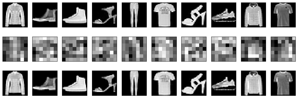
Display sample results
As usual, let’s see some sample results from the trained model.
def display_one_row(disp_images, offset, shape=(28, 28)):
  '''Display sample outputs in one row.'''
  for idx, test_image in enumerate(disp_images):
    plt.subplot(3, 10, offset + idx + 1)
    plt.xticks([])
    plt.yticks([])
    test_image = np.reshape(test_image, shape)
    plt.imshow(test_image, cmap='gray')


def display_results(disp_input_images, disp_encoded, disp_predicted, enc_shape=(8,4)):
  '''Displays the input, encoded, and decoded output values.'''
  plt.figure(figsize=(15, 5))
  display_one_row(disp_input_images, 0, shape=(28,28,))
  display_one_row(disp_encoded, 10, shape=enc_shape)
  display_one_row(disp_predicted, 20, shape=(28,28,))
# take 1 batch of the dataset
test_dataset = test_dataset.take(1)

# take the input images and put them in a list
output_samples = []
for input_image, image in tfds.as_numpy(test_dataset):
      output_samples = input_image

# pick 10 indices
idxs = np.array([1, 2, 3, 4, 5, 6, 7, 8, 9, 10])

# prepare test samples as a batch of 10 images
conv_output_samples = np.array(output_samples[idxs])
conv_output_samples = np.reshape(conv_output_samples, (10, 28, 28, 1))

# get the encoder ouput
encoded = convolutional_encoder_model.predict(conv_output_samples)

# get a prediction for some values in the dataset
predicted = convolutional_model.predict(conv_output_samples)

# display the samples, encodings and decoded values!
display_results(conv_output_samples, encoded, predicted, enc_shape=(7,7))
1/1 [==============================] - 0s 242ms/step
1/1 [==============================] - 0s 198ms/step