Coursera

Ungraded Lab: MNIST Autoencoder

You will now work on an autoencoder that works on the MNIST dataset. This will encode the inputs to lower resolution images. The decoder should then be able to generate the original input from this compressed representation.

Imports

try:
  # %tensorflow_version only exists in Colab.
  %tensorflow_version 2.x
except Exception:
  pass

import tensorflow as tf
import tensorflow_datasets as tfds

import numpy as np
import matplotlib.pyplot as plt

Colab only includes TensorFlow 2.x; %tensorflow_version has no effect.

Prepare the Dataset

You will load the MNIST data from TFDS into train and test sets. Let’s first define a preprocessing function for normalizing and flattening the images. Since we’ll be training an autoencoder, this will return image, image because the input will also be the target or label while training.

def map_image(image, label):
  '''Normalizes and flattens the image. Returns image as input and label.'''
  image = tf.cast(image, dtype=tf.float32)
  image = image / 255.0
  image = tf.reshape(image, shape=(784,))

  return image, image

# Load the train and test sets from TFDS

BATCH_SIZE = 128
SHUFFLE_BUFFER_SIZE = 1024

train_dataset = tfds.load('mnist', as_supervised=True, split="train")
train_dataset = train_dataset.map(map_image)
train_dataset = train_dataset.shuffle(SHUFFLE_BUFFER_SIZE).batch(BATCH_SIZE).repeat()

test_dataset = tfds.load('mnist', as_supervised=True, split="test")
test_dataset = test_dataset.map(map_image)
test_dataset = test_dataset.batch(BATCH_SIZE).repeat()

Downloading and preparing dataset 11.06 MiB (download: 11.06 MiB, generated: 21.00 MiB, total: 32.06 MiB) to /root/tensorflow_datasets/mnist/3.0.1...



Dl Completed...:   0%|          | 0/5 [00:00<?, ? file/s]


Dataset mnist downloaded and prepared to /root/tensorflow_datasets/mnist/3.0.1. Subsequent calls will reuse this data.

Build the Model

You will now build a simple autoencoder to ingest the data. Like before, the encoder will compress the input and reconstructs it in the decoder output.

def simple_autoencoder(inputs):
  '''Builds the encoder and decoder using Dense layers.'''
  encoder = tf.keras.layers.Dense(units=32, activation='relu')(inputs)
  decoder = tf.keras.layers.Dense(units=784, activation='sigmoid')(encoder)

  return encoder, decoder

# set the input shape
inputs =  tf.keras.layers.Input(shape=(784,))

# get the encoder and decoder output
encoder_output, decoder_output = simple_autoencoder(inputs)

# setup the encoder because you will visualize its output later
encoder_model = tf.keras.Model(inputs=inputs, outputs=encoder_output)

# setup the autoencoder
autoencoder_model = tf.keras.Model(inputs=inputs, outputs=decoder_output)

Compile the Model

You will setup the model for training. You can use binary crossentropy to measure the loss between pixel values that range from 0 (black) to 1 (white).

autoencoder_model.compile(
    optimizer=tf.keras.optimizers.Adam(),
    loss='binary_crossentropy')

Train the Model

train_steps = 60000 // BATCH_SIZE
simple_auto_history = autoencoder_model.fit(train_dataset, steps_per_epoch=train_steps, epochs=50)

Epoch 1/50
468/468 [==============================] - 18s 21ms/step - loss: 0.2292
Epoch 2/50
468/468 [==============================] - 4s 8ms/step - loss: 0.1424
Epoch 3/50
468/468 [==============================] - 5s 11ms/step - loss: 0.1199
Epoch 4/50
468/468 [==============================] - 4s 9ms/step - loss: 0.1086
Epoch 5/50
468/468 [==============================] - 5s 11ms/step - loss: 0.1019
Epoch 6/50
468/468 [==============================] - 4s 8ms/step - loss: 0.0980
Epoch 7/50
468/468 [==============================] - 3s 6ms/step - loss: 0.0959
Epoch 8/50
468/468 [==============================] - 3s 6ms/step - loss: 0.0949
Epoch 9/50
468/468 [==============================] - 3s 7ms/step - loss: 0.0944
Epoch 10/50
468/468 [==============================] - 4s 8ms/step - loss: 0.0941
Epoch 11/50
468/468 [==============================] - 3s 6ms/step - loss: 0.0939
Epoch 12/50
468/468 [==============================] - 3s 6ms/step - loss: 0.0937
Epoch 13/50
468/468 [==============================] - 3s 7ms/step - loss: 0.0936
Epoch 14/50
468/468 [==============================] - 3s 7ms/step - loss: 0.0935
Epoch 15/50
468/468 [==============================] - 3s 6ms/step - loss: 0.0934
Epoch 16/50
468/468 [==============================] - 3s 6ms/step - loss: 0.0933
Epoch 17/50
468/468 [==============================] - 4s 8ms/step - loss: 0.0932
Epoch 18/50
468/468 [==============================] - 3s 7ms/step - loss: 0.0932
Epoch 19/50
468/468 [==============================] - 3s 6ms/step - loss: 0.0931
Epoch 20/50
468/468 [==============================] - 3s 6ms/step - loss: 0.0931
Epoch 21/50
468/468 [==============================] - 3s 7ms/step - loss: 0.0931
Epoch 22/50
468/468 [==============================] - 3s 7ms/step - loss: 0.0930
Epoch 23/50
468/468 [==============================] - 3s 6ms/step - loss: 0.0929
Epoch 24/50
468/468 [==============================] - 4s 8ms/step - loss: 0.0930
Epoch 25/50
468/468 [==============================] - 4s 8ms/step - loss: 0.0929
Epoch 26/50
468/468 [==============================] - 3s 6ms/step - loss: 0.0929
Epoch 27/50
468/468 [==============================] - 3s 6ms/step - loss: 0.0928
Epoch 28/50
468/468 [==============================] - 3s 6ms/step - loss: 0.0928
Epoch 29/50
468/468 [==============================] - 4s 8ms/step - loss: 0.0928
Epoch 30/50
468/468 [==============================] - 3s 7ms/step - loss: 0.0928
Epoch 31/50
468/468 [==============================] - 3s 6ms/step - loss: 0.0928
Epoch 32/50
468/468 [==============================] - 3s 6ms/step - loss: 0.0927
Epoch 33/50
468/468 [==============================] - 4s 10ms/step - loss: 0.0927
Epoch 34/50
468/468 [==============================] - 3s 6ms/step - loss: 0.0927
Epoch 35/50
468/468 [==============================] - 3s 6ms/step - loss: 0.0927
Epoch 36/50
468/468 [==============================] - 4s 9ms/step - loss: 0.0927
Epoch 37/50
468/468 [==============================] - 4s 8ms/step - loss: 0.0927
Epoch 38/50
468/468 [==============================] - 3s 6ms/step - loss: 0.0927
Epoch 39/50
468/468 [==============================] - 3s 6ms/step - loss: 0.0926
Epoch 40/50
468/468 [==============================] - 3s 7ms/step - loss: 0.0926
Epoch 41/50
468/468 [==============================] - 3s 7ms/step - loss: 0.0926
Epoch 42/50
468/468 [==============================] - 3s 6ms/step - loss: 0.0926
Epoch 43/50
468/468 [==============================] - 3s 6ms/step - loss: 0.0926
Epoch 44/50
468/468 [==============================] - 3s 7ms/step - loss: 0.0926
Epoch 45/50
468/468 [==============================] - 4s 8ms/step - loss: 0.0926
Epoch 46/50
468/468 [==============================] - 3s 6ms/step - loss: 0.0926
Epoch 47/50
468/468 [==============================] - 3s 6ms/step - loss: 0.0925
Epoch 48/50
468/468 [==============================] - 3s 7ms/step - loss: 0.0925
Epoch 49/50
468/468 [==============================] - 4s 8ms/step - loss: 0.0926
Epoch 50/50
468/468 [==============================] - 3s 6ms/step - loss: 0.0925

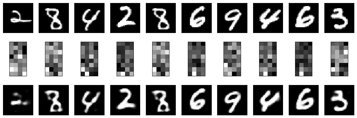
Display sample results

You can now visualize the results. The utility functions below will help in plotting the encoded and decoded values.

def display_one_row(disp_images, offset, shape=(28, 28)):
  '''Display sample outputs in one row.'''
  for idx, test_image in enumerate(disp_images):
    plt.subplot(3, 10, offset + idx + 1)
    plt.xticks([])
    plt.yticks([])
    test_image = np.reshape(test_image, shape)
    plt.imshow(test_image, cmap='gray')


def display_results(disp_input_images, disp_encoded, disp_predicted, enc_shape=(8,4)):
  '''Displays the input, encoded, and decoded output values.'''
  plt.figure(figsize=(15, 5))
  display_one_row(disp_input_images, 0, shape=(28,28,))
  display_one_row(disp_encoded, 10, shape=enc_shape)
  display_one_row(disp_predicted, 20, shape=(28,28,))

# take 1 batch of the dataset
test_dataset = test_dataset.take(1)

# take the input images and put them in a list
output_samples = []
for input_image, image in tfds.as_numpy(test_dataset):
      output_samples = input_image

# pick 10 random numbers to be used as indices to the list above
idxs = np.random.choice(BATCH_SIZE, size=10)

# get the encoder output
encoded_predicted = encoder_model.predict(test_dataset)

# get a prediction for the test batch
simple_predicted = autoencoder_model.predict(test_dataset)

# display the 10 samples, encodings and decoded values!
display_results(output_samples[idxs], encoded_predicted[idxs], simple_predicted[idxs])

1/1 [==============================] - 0s 111ms/step
1/1 [==============================] - 0s 87ms/step