Coursera

Week 1: Multiple Output Models using the Keras Functional API

Welcome to the first programming assignment of the course! Your task will be to use the Keras functional API to train a model to predict two outputs. For this lab, you will use the Wine Quality Dataset from the UCI machine learning repository. It has separate datasets for red wine and white wine.

Normally, the wines are classified into one of the quality ratings specified in the attributes. In this exercise, you will combine the two datasets to predict the wine quality and whether the wine is red or white solely from the attributes.

You will model wine quality estimations as a regression problem and wine type detection as a binary classification problem.

Please complete sections that are marked (TODO)

Imports

import tensorflow as tf
from tensorflow.keras.models import Model
from tensorflow.keras.layers import Dense, Input

import numpy as np
import matplotlib.pyplot as plt
import pandas as pd
from sklearn.model_selection import train_test_split
from sklearn.metrics import confusion_matrix, ConfusionMatrixDisplay
import itertools

import utils

Load Dataset

You will now load the dataset from the UCI Machine Learning Repository which are already saved in your workspace (Note: For successful grading, please do not modify the default string set to the URI variable below).

Pre-process the white wine dataset (TODO)

You will add a new column named is_red in your dataframe to indicate if the wine is white or red.

In the white wine dataset, you will fill the column is_red with zeros (0).

# Please uncomment all lines in this cell and replace those marked with `# YOUR CODE HERE`.
# You can select all lines in this code cell with Ctrl+A (Windows/Linux) or Cmd+A (Mac), then press Ctrl+/ (Windows/Linux) or Cmd+/ (Mac) to uncomment.



# URL of the white wine dataset
URI = './winequality-white.csv'

# load the dataset from the URL
white_df = pd.read_csv(URI, sep=";")

# fill the `is_red` column with zeros.
white_df["is_red"] = 0

# keep only the first of duplicate items
white_df = white_df.drop_duplicates(keep='first')

# You can click `File -> Open` in the menu above and open the `utils.py` file 
# in case you want to inspect the unit tests being used for each graded function.

utils.test_white_df(white_df)

[92m All public tests passed

print(white_df.alcohol[0])
print(white_df.alcohol[100])

# EXPECTED OUTPUT
# 8.8
# 9.1

8.8
9.1

Pre-process the red wine dataset (TODO)

In the red wine dataset, you will fill in the column is_red with ones (1).

# Please uncomment all lines in this cell and replace those marked with `# YOUR CODE HERE`.
# You can select all lines in this code cell with Ctrl+A (Windows/Linux) or Cmd+A (Mac), then press Ctrl+/ (Windows/Linux) or Cmd+/ (Mac) to uncomment.



# URL of the red wine dataset
URI = './winequality-red.csv'

# load the dataset from the URL
red_df = pd.read_csv(URI, sep=";")

# fill the `is_red` column with ones.
red_df["is_red"] = 1

# keep only the first of duplicate items
red_df = red_df.drop_duplicates(keep='first')

utils.test_red_df(red_df)

[92m All public tests passed

print(red_df.alcohol[0])
print(red_df.alcohol[100])

# EXPECTED OUTPUT
# 9.4
# 10.2

9.4
10.2

Concatenate the datasets

Next, concatenate the red and white wine dataframes.

df = pd.concat([red_df, white_df], ignore_index=True)

print(df.alcohol[0])
print(df.alcohol[100])

# EXPECTED OUTPUT
# 9.4
# 9.5

9.4
9.5

In a real-world scenario, you should shuffle the data. For this assignment however, you are not going to do that because the grader needs to test with deterministic data. If you want the code to do it after you’ve gotten your grade for this notebook, we left the commented line below for reference

#df = df.iloc[np.random.permutation(len(df))]

This will chart the quality of the wines.

df['quality'].hist(bins=20);

png

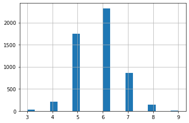
Imbalanced data (TODO)

You can see from the plot above that the wine quality dataset is imbalanced.

Since there are very few observations with quality equal to 3, 4, 8 and 9, you can drop these observations from your dataset.
You can do this by removing data belonging to all classes except those > 4 and < 8.

# Please uncomment all lines in this cell and replace those marked with `# YOUR CODE HERE`.
# You can select all lines in this code cell with Ctrl+A (Windows/Linux) or Cmd+A (Mac), then press Ctrl+/ (Windows/Linux) or Cmd+/ (Mac) to uncomment.



# get data with wine quality greater than 4 and less than 8
df = df[(df['quality'] > 4) & (df['quality'] < 8)]

# reset index and drop the old one
df = df.reset_index(drop=True)

utils.test_df_drop(df)

[92m All public tests passed

print(df.alcohol[0])
print(df.alcohol[100])

# EXPECTED OUTPUT
# 9.4
# 10.9

9.4
10.9

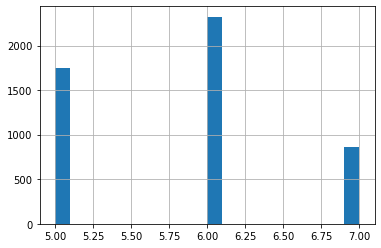
You can plot again to see the new range of data and quality

df['quality'].hist(bins=20);

png

Train Test Split (TODO)

Next, you can split the datasets into training, test and validation datasets.

The data frame should be split 80:20 into train and test sets.
The resulting train should then be split 80:20 into train and val sets.
The train_test_split parameter test_size takes a float value that ranges between 0. and 1, and represents the proportion of the dataset that is allocated to the test set. The rest of the data is allocated to the training set.

# Please uncomment all lines in this cell and replace those marked with `# YOUR CODE HERE`.
# You can select all lines in this code cell with Ctrl+A (Windows/Linux) or Cmd+A (Mac), then press Ctrl+/ (Windows/Linux) or Cmd+/ (Mac) to uncomment.

# Please do not change the random_state parameter. This is needed for grading.

# split df into 80:20 train and test sets
train, test = train_test_split(df, test_size=.2, random_state = 1)
                               
# split train into 80:20 train and val sets
train, val = train_test_split(train, test_size=.2, random_state = 1)

utils.test_data_sizes(train.size, test.size, val.size)

[92m All public tests passed

Here’s where you can explore the training stats. You can pop the labels ‘is_red’ and ‘quality’ from the data as these will be used as the labels

train_stats = train.describe()
train_stats.pop('is_red')
train_stats.pop('quality')
train_stats = train_stats.transpose()

Explore the training stats!

train_stats

.dataframe tbody tr th {
    vertical-align: top;
}

.dataframe thead th {
    text-align: right;
}

	count	mean	std	min	25%	50%	75%	max
fixed acidity	3155.0	7.221616	1.325297	3.80000	6.40000	7.00000	7.7000	15.60000
volatile acidity	3155.0	0.338929	0.162476	0.08000	0.23000	0.29000	0.4000	1.24000
citric acid	3155.0	0.321569	0.147970	0.00000	0.25000	0.31000	0.4000	1.66000
residual sugar	3155.0	5.155911	4.639632	0.60000	1.80000	2.80000	7.6500	65.80000
chlorides	3155.0	0.056976	0.036802	0.01200	0.03800	0.04700	0.0660	0.61100
free sulfur dioxide	3155.0	30.388590	17.236784	1.00000	17.00000	28.00000	41.0000	131.00000
total sulfur dioxide	3155.0	115.062282	56.706617	6.00000	75.00000	117.00000	156.0000	344.00000
density	3155.0	0.994633	0.003005	0.98711	0.99232	0.99481	0.9968	1.03898
pH	3155.0	3.223201	0.161272	2.72000	3.11000	3.21000	3.3300	4.01000
sulphates	3155.0	0.534051	0.149149	0.22000	0.43000	0.51000	0.6000	1.95000
alcohol	3155.0	10.504466	1.154654	8.50000	9.50000	10.30000	11.3000	14.00000

Get the labels (TODO)

The features and labels are currently in the same dataframe.

You will want to store the label columns is_red and quality separately from the feature columns.
The following function, format_output, gets these two columns from the dataframe (it’s given to you).
format_output also formats the data into numpy arrays.
Please use the format_output and apply it to the train, val and test sets to get dataframes for the labels.

def format_output(data):
    is_red = data.pop('is_red')
    is_red = np.array(is_red)
    quality = data.pop('quality')
    quality = np.array(quality)
    return (quality, is_red)

# Please uncomment all lines in this cell and replace those marked with `# YOUR CODE HERE`.
# You can select all lines in this code cell with Ctrl+A (Windows/Linux) or Cmd+A (Mac), then press Ctrl+/ (Windows/Linux) or Cmd+/ (Mac) to uncomment.



# format the output of the train set
train_Y = format_output(train)

# format the output of the val set
val_Y = format_output(val)
    
# format the output of the test set
test_Y = format_output(test)

utils.test_format_output(df, train_Y, val_Y, test_Y)

[92m All public tests passed

Notice that after you get the labels, the train, val and test dataframes no longer contain the label columns, and contain just the feature columns.

This is because you used .pop in the format_output function.

train.head()

.dataframe tbody tr th {
    vertical-align: top;
}

.dataframe thead th {
    text-align: right;
}

	fixed acidity	volatile acidity	citric acid	residual sugar	chlorides	free sulfur dioxide	total sulfur dioxide	density	pH	sulphates	alcohol
225	7.5	0.65	0.18	7.0	0.088	27.0	94.0	0.99915	3.38	0.77	9.4
3557	6.3	0.27	0.29	12.2	0.044	59.0	196.0	0.99782	3.14	0.40	8.8
3825	8.8	0.27	0.25	5.0	0.024	52.0	99.0	0.99250	2.87	0.49	11.4
1740	6.4	0.45	0.07	1.1	0.030	10.0	131.0	0.99050	2.97	0.28	10.8
1221	7.2	0.53	0.13	2.0	0.058	18.0	22.0	0.99573	3.21	0.68	9.9

Normalize the data (TODO)

Next, you can normalize the data, x, using the formula: $$x_{norm} = \frac{x - \mu}{\sigma}$$

The norm function is defined for you.
Please apply the norm function to normalize the dataframes that contains the feature columns of train, val and test sets.

def norm(x):
    return (x - train_stats['mean']) / train_stats['std']

# Please uncomment all lines in this cell and replace those marked with `# YOUR CODE HERE`.
# You can select all lines in this code cell with Ctrl+A (Windows/Linux) or Cmd+A (Mac), then press Ctrl+/ (Windows/Linux) or Cmd+/ (Mac) to uncomment.



# normalize the train set
norm_train_X = norm(train)
    
# normalize the val set
norm_val_X = norm(val)
    
# normalize the test set
norm_test_X = norm(test)

utils.test_norm(norm_train_X, norm_val_X, norm_test_X, train, val, test)

[92m All public tests passed

Define the Model (TODO)

Define the model using the functional API. The base model will be 2 Dense layers of 128 neurons each, and have the 'relu' activation.

Check out the documentation for tf.keras.layers.Dense

# Please uncomment all lines in this cell and replace those marked with `# YOUR CODE HERE`.
# You can select all lines in this code cell with Ctrl+A (Windows/Linux) or Cmd+A (Mac), then press Ctrl+/ (Windows/Linux) or Cmd+/ (Mac) to uncomment.

def base_model(inputs):
    
    # connect a Dense layer with 128 neurons and a relu activation
    x = tf.keras.layers.Dense(128, activation="relu")(inputs)
    
    # connect another Dense layer with 128 neurons and a relu activation
    x = tf.keras.layers.Dense(128, activation="relu")(x)
    return x

utils.test_base_model(base_model)

[92m All public tests passed

Define output layers of the model (TODO)

You will add output layers to the base model.

The model will need two outputs.

One output layer will predict wine quality, which is a numeric value.

Define a Dense layer with 1 neuron.
Since this is a regression output, the activation can be left as its default value None.

The other output layer will predict the wine type, which is either red 1 or not red 0 (white).

Define a Dense layer with 1 neuron.
Since there are two possible categories, you can use a sigmoid activation for binary classification.

Define the Model

Define the Model object, and set the following parameters:
- inputs: pass in the inputs to the model as a list.
- outputs: pass in a list of the outputs that you just defined: wine quality, then wine type.
- Note: please list the wine quality before wine type in the outputs, as this will affect the calculated loss if you choose the other order.

# Please uncomment all lines in this cell and replace those marked with `# YOUR CODE HERE`.
# You can select all lines in this code cell with Ctrl+A (Windows/Linux) or Cmd+A (Mac), then press Ctrl+/ (Windows/Linux) or Cmd+/ (Mac) to uncomment.



def final_model(inputs):
    
    # get the base model
    x = base_model(inputs)

    # connect the output Dense layer for regression
    wine_quality = Dense(units='1', name='wine_quality')(x)

    # connect the output Dense layer for classification. this will use a sigmoid activation.
    wine_type = Dense(units='1', activation="sigmoid", name='wine_type')(x)

    # define the model using the input and output layers
    model = Model(inputs=inputs, outputs=[wine_quality, wine_type])

    return model

utils.test_final_model(final_model)

[92m All public tests passed

Compiling the Model

Next, compile the model. When setting the loss parameter of model.compile, you’re setting the loss for each of the two outputs (wine quality and wine type).

To set more than one loss, use a dictionary of key-value pairs.

You can look at the docs for the losses here.
- Note: For the desired spelling, please look at the “Functions” section of the documentation and not the “classes” section on that same page.
wine_type: Since you will be performing binary classification on wine type, you should use the binary crossentropy loss function for it. Please pass this in as a string.
- Hint, this should be all lowercase. In the documentation, you’ll see this under the “Functions” section, not the “Classes” section.
wine_quality: since this is a regression output, use the mean squared error. Please pass it in as a string, all lowercase.
- Hint: You may notice that there are two aliases for mean squared error. Please use the shorter name.

You will also set the metric for each of the two outputs. Again, to set metrics for two or more outputs, use a dictionary with key value pairs.

The metrics documentation is linked here.
For the wine type, please set it to accuracy as a string, all lowercase.
For wine quality, please use the root mean squared error. Instead of a string, you’ll set it to an instance of the class RootMeanSquaredError, which belongs to the tf.keras.metrics module.

Note: If you see the error message

Exception: wine quality loss function is incorrect.

Please also check your other losses and metrics, as the error may be caused by the other three key-value pairs and not the wine quality loss.

# Please uncomment all lines in this cell and replace those marked with `# YOUR CODE HERE`.
# You can select all lines in this code cell with Ctrl+A (Windows/Linux) or Cmd+A (Mac), then press Ctrl+/ (Windows/Linux) or Cmd+/ (Mac) to uncomment.



inputs = tf.keras.layers.Input(shape=(11,))
rms = tf.keras.optimizers.RMSprop(lr=0.0001)
model = final_model(inputs)

model.compile(optimizer=rms, 
              loss = {'wine_type' : "binary_crossentropy",
                      'wine_quality' : "mean_squared_error"
                     },
              metrics = {'wine_type' : "accuracy",
                         'wine_quality': tf.keras.metrics.RootMeanSquaredError()
                       }
             )

utils.test_model_compile(model)

[92m All public tests passed

Training the Model (TODO)

Fit the model to the training inputs and outputs.

Check the documentation for model.fit.
Remember to use the normalized training set as inputs.
For the validation data, please use the normalized validation set.

Important: Please do not increase the number of epochs below. This is to avoid the grader from timing out. You can increase it once you have submitted your work.

# Please uncomment all lines in this cell and replace those marked with `# YOUR CODE HERE`.
# You can select all lines in this code cell with Ctrl+A (Windows/Linux) or Cmd+A (Mac), then press Ctrl+/ (Windows/Linux) or Cmd+/ (Mac) to uncomment.

history = model.fit(norm_train_X, train_Y,
                    epochs = 40, validation_data=(norm_val_X, val_Y))

Train on 3155 samples, validate on 789 samples
Epoch 1/40
3155/3155 [==============================] - 1s 388us/sample - loss: 26.0949 - wine_quality_loss: 25.3988 - wine_type_loss: 0.6655 - wine_quality_root_mean_squared_error: 5.0427 - wine_type_accuracy: 0.5743 - val_loss: 18.5594 - val_wine_quality_loss: 17.9177 - val_wine_type_loss: 0.6556 - val_wine_quality_root_mean_squared_error: 4.2314 - val_wine_type_accuracy: 0.6210
Epoch 2/40
3155/3155 [==============================] - 0s 102us/sample - loss: 12.7250 - wine_quality_loss: 12.0808 - wine_type_loss: 0.6259 - wine_quality_root_mean_squared_error: 3.4784 - wine_type_accuracy: 0.6995 - val_loss: 7.5900 - val_wine_quality_loss: 7.0423 - val_wine_type_loss: 0.5973 - val_wine_quality_root_mean_squared_error: 2.6445 - val_wine_type_accuracy: 0.7782
Epoch 3/40
3155/3155 [==============================] - 0s 99us/sample - loss: 5.0478 - wine_quality_loss: 4.4990 - wine_type_loss: 0.5444 - wine_quality_root_mean_squared_error: 2.1221 - wine_type_accuracy: 0.8371 - val_loss: 3.1732 - val_wine_quality_loss: 2.7383 - val_wine_type_loss: 0.4959 - val_wine_quality_root_mean_squared_error: 1.6364 - val_wine_type_accuracy: 0.8555
Epoch 4/40
3155/3155 [==============================] - 0s 113us/sample - loss: 2.9146 - wine_quality_loss: 2.4767 - wine_type_loss: 0.4343 - wine_quality_root_mean_squared_error: 1.5748 - wine_type_accuracy: 0.8704 - val_loss: 2.4602 - val_wine_quality_loss: 2.1188 - val_wine_type_loss: 0.3854 - val_wine_quality_root_mean_squared_error: 1.4405 - val_wine_type_accuracy: 0.8847
Epoch 5/40
3155/3155 [==============================] - 0s 97us/sample - loss: 2.3504 - wine_quality_loss: 2.0118 - wine_type_loss: 0.3329 - wine_quality_root_mean_squared_error: 1.4202 - wine_type_accuracy: 0.9185 - val_loss: 2.0869 - val_wine_quality_loss: 1.8195 - val_wine_type_loss: 0.2943 - val_wine_quality_root_mean_squared_error: 1.3389 - val_wine_type_accuracy: 0.9417
Epoch 6/40
3155/3155 [==============================] - 0s 97us/sample - loss: 2.0094 - wine_quality_loss: 1.7505 - wine_type_loss: 0.2542 - wine_quality_root_mean_squared_error: 1.3248 - wine_type_accuracy: 0.9642 - val_loss: 1.8331 - val_wine_quality_loss: 1.6284 - val_wine_type_loss: 0.2238 - val_wine_quality_root_mean_squared_error: 1.2685 - val_wine_type_accuracy: 0.9747
Epoch 7/40
3155/3155 [==============================] - 0s 96us/sample - loss: 1.7793 - wine_quality_loss: 1.5893 - wine_type_loss: 0.1933 - wine_quality_root_mean_squared_error: 1.2594 - wine_type_accuracy: 0.9784 - val_loss: 1.6532 - val_wine_quality_loss: 1.4949 - val_wine_type_loss: 0.1712 - val_wine_quality_root_mean_squared_error: 1.2173 - val_wine_type_accuracy: 0.9823
Epoch 8/40
3155/3155 [==============================] - 0s 94us/sample - loss: 1.6099 - wine_quality_loss: 1.4571 - wine_type_loss: 0.1499 - wine_quality_root_mean_squared_error: 1.2082 - wine_type_accuracy: 0.9845 - val_loss: 1.5201 - val_wine_quality_loss: 1.3940 - val_wine_type_loss: 0.1346 - val_wine_quality_root_mean_squared_error: 1.1770 - val_wine_type_accuracy: 0.9886
Epoch 9/40
3155/3155 [==============================] - 0s 96us/sample - loss: 1.4854 - wine_quality_loss: 1.3616 - wine_type_loss: 0.1203 - wine_quality_root_mean_squared_error: 1.1683 - wine_type_accuracy: 0.9883 - val_loss: 1.3933 - val_wine_quality_loss: 1.2914 - val_wine_type_loss: 0.1080 - val_wine_quality_root_mean_squared_error: 1.1336 - val_wine_type_accuracy: 0.9886
Epoch 10/40
3155/3155 [==============================] - 0s 94us/sample - loss: 1.3808 - wine_quality_loss: 1.2840 - wine_type_loss: 0.0994 - wine_quality_root_mean_squared_error: 1.1319 - wine_type_accuracy: 0.9899 - val_loss: 1.2996 - val_wine_quality_loss: 1.2137 - val_wine_type_loss: 0.0894 - val_wine_quality_root_mean_squared_error: 1.1000 - val_wine_type_accuracy: 0.9899
Epoch 11/40
3155/3155 [==============================] - 0s 93us/sample - loss: 1.2834 - wine_quality_loss: 1.2010 - wine_type_loss: 0.0842 - wine_quality_root_mean_squared_error: 1.0950 - wine_type_accuracy: 0.9902 - val_loss: 1.2191 - val_wine_quality_loss: 1.1465 - val_wine_type_loss: 0.0762 - val_wine_quality_root_mean_squared_error: 1.0689 - val_wine_type_accuracy: 0.9911
Epoch 12/40
3155/3155 [==============================] - 0s 93us/sample - loss: 1.2152 - wine_quality_loss: 1.1423 - wine_type_loss: 0.0733 - wine_quality_root_mean_squared_error: 1.0685 - wine_type_accuracy: 0.9908 - val_loss: 1.1442 - val_wine_quality_loss: 1.0794 - val_wine_type_loss: 0.0670 - val_wine_quality_root_mean_squared_error: 1.0377 - val_wine_type_accuracy: 0.9911
Epoch 13/40
3155/3155 [==============================] - 0s 94us/sample - loss: 1.1438 - wine_quality_loss: 1.0791 - wine_type_loss: 0.0657 - wine_quality_root_mean_squared_error: 1.0383 - wine_type_accuracy: 0.9908 - val_loss: 1.0789 - val_wine_quality_loss: 1.0203 - val_wine_type_loss: 0.0596 - val_wine_quality_root_mean_squared_error: 1.0095 - val_wine_type_accuracy: 0.9924
Epoch 14/40
3155/3155 [==============================] - 0s 95us/sample - loss: 1.0794 - wine_quality_loss: 1.0201 - wine_type_loss: 0.0600 - wine_quality_root_mean_squared_error: 1.0098 - wine_type_accuracy: 0.9908 - val_loss: 1.0191 - val_wine_quality_loss: 0.9655 - val_wine_type_loss: 0.0543 - val_wine_quality_root_mean_squared_error: 0.9821 - val_wine_type_accuracy: 0.9937
Epoch 15/40
3155/3155 [==============================] - 0s 93us/sample - loss: 1.0237 - wine_quality_loss: 0.9678 - wine_type_loss: 0.0551 - wine_quality_root_mean_squared_error: 0.9841 - wine_type_accuracy: 0.9908 - val_loss: 0.9673 - val_wine_quality_loss: 0.9170 - val_wine_type_loss: 0.0505 - val_wine_quality_root_mean_squared_error: 0.9573 - val_wine_type_accuracy: 0.9937
Epoch 16/40
3155/3155 [==============================] - 0s 93us/sample - loss: 0.9668 - wine_quality_loss: 0.9145 - wine_type_loss: 0.0516 - wine_quality_root_mean_squared_error: 0.9566 - wine_type_accuracy: 0.9908 - val_loss: 0.9151 - val_wine_quality_loss: 0.8674 - val_wine_type_loss: 0.0476 - val_wine_quality_root_mean_squared_error: 0.9312 - val_wine_type_accuracy: 0.9937
Epoch 17/40
3155/3155 [==============================] - 0s 79us/sample - loss: 0.9208 - wine_quality_loss: 0.8703 - wine_type_loss: 0.0490 - wine_quality_root_mean_squared_error: 0.9337 - wine_type_accuracy: 0.9908 - val_loss: 0.8664 - val_wine_quality_loss: 0.8213 - val_wine_type_loss: 0.0450 - val_wine_quality_root_mean_squared_error: 0.9062 - val_wine_type_accuracy: 0.9924
Epoch 18/40
3155/3155 [==============================] - 0s 93us/sample - loss: 0.8762 - wine_quality_loss: 0.8302 - wine_type_loss: 0.0469 - wine_quality_root_mean_squared_error: 0.9108 - wine_type_accuracy: 0.9908 - val_loss: 0.8200 - val_wine_quality_loss: 0.7765 - val_wine_type_loss: 0.0430 - val_wine_quality_root_mean_squared_error: 0.8812 - val_wine_type_accuracy: 0.9924
Epoch 19/40
3155/3155 [==============================] - 0s 94us/sample - loss: 0.8323 - wine_quality_loss: 0.7859 - wine_type_loss: 0.0448 - wine_quality_root_mean_squared_error: 0.8873 - wine_type_accuracy: 0.9908 - val_loss: 0.7808 - val_wine_quality_loss: 0.7385 - val_wine_type_loss: 0.0417 - val_wine_quality_root_mean_squared_error: 0.8595 - val_wine_type_accuracy: 0.9924
Epoch 20/40
3155/3155 [==============================] - 0s 92us/sample - loss: 0.7918 - wine_quality_loss: 0.7472 - wine_type_loss: 0.0434 - wine_quality_root_mean_squared_error: 0.8651 - wine_type_accuracy: 0.9911 - val_loss: 0.7458 - val_wine_quality_loss: 0.7047 - val_wine_type_loss: 0.0401 - val_wine_quality_root_mean_squared_error: 0.8398 - val_wine_type_accuracy: 0.9937
Epoch 21/40
3155/3155 [==============================] - 0s 94us/sample - loss: 0.7550 - wine_quality_loss: 0.7138 - wine_type_loss: 0.0419 - wine_quality_root_mean_squared_error: 0.8444 - wine_type_accuracy: 0.9908 - val_loss: 0.7139 - val_wine_quality_loss: 0.6741 - val_wine_type_loss: 0.0390 - val_wine_quality_root_mean_squared_error: 0.8213 - val_wine_type_accuracy: 0.9937
Epoch 22/40
3155/3155 [==============================] - 0s 93us/sample - loss: 0.7217 - wine_quality_loss: 0.6807 - wine_type_loss: 0.0406 - wine_quality_root_mean_squared_error: 0.8252 - wine_type_accuracy: 0.9908 - val_loss: 0.6781 - val_wine_quality_loss: 0.6388 - val_wine_type_loss: 0.0381 - val_wine_quality_root_mean_squared_error: 0.7997 - val_wine_type_accuracy: 0.9937
Epoch 23/40
3155/3155 [==============================] - 0s 94us/sample - loss: 0.6855 - wine_quality_loss: 0.6473 - wine_type_loss: 0.0399 - wine_quality_root_mean_squared_error: 0.8036 - wine_type_accuracy: 0.9921 - val_loss: 0.6477 - val_wine_quality_loss: 0.6095 - val_wine_type_loss: 0.0371 - val_wine_quality_root_mean_squared_error: 0.7812 - val_wine_type_accuracy: 0.9949
Epoch 24/40
3155/3155 [==============================] - 0s 96us/sample - loss: 0.6536 - wine_quality_loss: 0.6147 - wine_type_loss: 0.0387 - wine_quality_root_mean_squared_error: 0.7841 - wine_type_accuracy: 0.9921 - val_loss: 0.6223 - val_wine_quality_loss: 0.5848 - val_wine_type_loss: 0.0367 - val_wine_quality_root_mean_squared_error: 0.7650 - val_wine_type_accuracy: 0.9949
Epoch 25/40
3155/3155 [==============================] - 0s 91us/sample - loss: 0.6278 - wine_quality_loss: 0.5897 - wine_type_loss: 0.0381 - wine_quality_root_mean_squared_error: 0.7680 - wine_type_accuracy: 0.9918 - val_loss: 0.5912 - val_wine_quality_loss: 0.5540 - val_wine_type_loss: 0.0361 - val_wine_quality_root_mean_squared_error: 0.7448 - val_wine_type_accuracy: 0.9949
Epoch 26/40
3155/3155 [==============================] - 0s 94us/sample - loss: 0.6031 - wine_quality_loss: 0.5659 - wine_type_loss: 0.0371 - wine_quality_root_mean_squared_error: 0.7522 - wine_type_accuracy: 0.9921 - val_loss: 0.5657 - val_wine_quality_loss: 0.5289 - val_wine_type_loss: 0.0356 - val_wine_quality_root_mean_squared_error: 0.7279 - val_wine_type_accuracy: 0.9949
Epoch 27/40
3155/3155 [==============================] - 0s 92us/sample - loss: 0.5761 - wine_quality_loss: 0.5389 - wine_type_loss: 0.0366 - wine_quality_root_mean_squared_error: 0.7345 - wine_type_accuracy: 0.9924 - val_loss: 0.5580 - val_wine_quality_loss: 0.5218 - val_wine_type_loss: 0.0351 - val_wine_quality_root_mean_squared_error: 0.7228 - val_wine_type_accuracy: 0.9949
Epoch 28/40
3155/3155 [==============================] - 0s 78us/sample - loss: 0.5550 - wine_quality_loss: 0.5186 - wine_type_loss: 0.0359 - wine_quality_root_mean_squared_error: 0.7205 - wine_type_accuracy: 0.9927 - val_loss: 0.5256 - val_wine_quality_loss: 0.4900 - val_wine_type_loss: 0.0348 - val_wine_quality_root_mean_squared_error: 0.7003 - val_wine_type_accuracy: 0.9949
Epoch 29/40
3155/3155 [==============================] - 0s 94us/sample - loss: 0.5339 - wine_quality_loss: 0.4977 - wine_type_loss: 0.0369 - wine_quality_root_mean_squared_error: 0.7061 - wine_type_accuracy: 0.9927 - val_loss: 0.5052 - val_wine_quality_loss: 0.4698 - val_wine_type_loss: 0.0343 - val_wine_quality_root_mean_squared_error: 0.6859 - val_wine_type_accuracy: 0.9949
Epoch 30/40
3155/3155 [==============================] - 0s 94us/sample - loss: 0.5152 - wine_quality_loss: 0.4793 - wine_type_loss: 0.0349 - wine_quality_root_mean_squared_error: 0.6930 - wine_type_accuracy: 0.9930 - val_loss: 0.4843 - val_wine_quality_loss: 0.4492 - val_wine_type_loss: 0.0340 - val_wine_quality_root_mean_squared_error: 0.6708 - val_wine_type_accuracy: 0.9949
Epoch 31/40
3155/3155 [==============================] - 0s 93us/sample - loss: 0.4960 - wine_quality_loss: 0.4606 - wine_type_loss: 0.0343 - wine_quality_root_mean_squared_error: 0.6794 - wine_type_accuracy: 0.9927 - val_loss: 0.4705 - val_wine_quality_loss: 0.4359 - val_wine_type_loss: 0.0335 - val_wine_quality_root_mean_squared_error: 0.6607 - val_wine_type_accuracy: 0.9949
Epoch 32/40
3155/3155 [==============================] - 0s 92us/sample - loss: 0.4810 - wine_quality_loss: 0.4475 - wine_type_loss: 0.0338 - wine_quality_root_mean_squared_error: 0.6686 - wine_type_accuracy: 0.9927 - val_loss: 0.4581 - val_wine_quality_loss: 0.4237 - val_wine_type_loss: 0.0332 - val_wine_quality_root_mean_squared_error: 0.6516 - val_wine_type_accuracy: 0.9949
Epoch 33/40
3155/3155 [==============================] - 0s 92us/sample - loss: 0.4655 - wine_quality_loss: 0.4314 - wine_type_loss: 0.0334 - wine_quality_root_mean_squared_error: 0.6573 - wine_type_accuracy: 0.9927 - val_loss: 0.4450 - val_wine_quality_loss: 0.4108 - val_wine_type_loss: 0.0330 - val_wine_quality_root_mean_squared_error: 0.6416 - val_wine_type_accuracy: 0.9949
Epoch 34/40
3155/3155 [==============================] - 0s 90us/sample - loss: 0.4522 - wine_quality_loss: 0.4183 - wine_type_loss: 0.0332 - wine_quality_root_mean_squared_error: 0.6474 - wine_type_accuracy: 0.9927 - val_loss: 0.4368 - val_wine_quality_loss: 0.4024 - val_wine_type_loss: 0.0327 - val_wine_quality_root_mean_squared_error: 0.6353 - val_wine_type_accuracy: 0.9949
Epoch 35/40
3155/3155 [==============================] - 0s 78us/sample - loss: 0.4424 - wine_quality_loss: 0.4092 - wine_type_loss: 0.0327 - wine_quality_root_mean_squared_error: 0.6400 - wine_type_accuracy: 0.9927 - val_loss: 0.4244 - val_wine_quality_loss: 0.3903 - val_wine_type_loss: 0.0326 - val_wine_quality_root_mean_squared_error: 0.6257 - val_wine_type_accuracy: 0.9949
Epoch 36/40
3155/3155 [==============================] - 0s 93us/sample - loss: 0.4305 - wine_quality_loss: 0.3985 - wine_type_loss: 0.0323 - wine_quality_root_mean_squared_error: 0.6310 - wine_type_accuracy: 0.9930 - val_loss: 0.4123 - val_wine_quality_loss: 0.3786 - val_wine_type_loss: 0.0324 - val_wine_quality_root_mean_squared_error: 0.6160 - val_wine_type_accuracy: 0.9949
Epoch 37/40
3155/3155 [==============================] - 0s 91us/sample - loss: 0.4202 - wine_quality_loss: 0.3881 - wine_type_loss: 0.0319 - wine_quality_root_mean_squared_error: 0.6231 - wine_type_accuracy: 0.9930 - val_loss: 0.4123 - val_wine_quality_loss: 0.3789 - val_wine_type_loss: 0.0323 - val_wine_quality_root_mean_squared_error: 0.6161 - val_wine_type_accuracy: 0.9949
Epoch 38/40
3155/3155 [==============================] - 0s 93us/sample - loss: 0.4112 - wine_quality_loss: 0.3794 - wine_type_loss: 0.0316 - wine_quality_root_mean_squared_error: 0.6160 - wine_type_accuracy: 0.9933 - val_loss: 0.3978 - val_wine_quality_loss: 0.3647 - val_wine_type_loss: 0.0320 - val_wine_quality_root_mean_squared_error: 0.6045 - val_wine_type_accuracy: 0.9949
Epoch 39/40
3155/3155 [==============================] - 0s 98us/sample - loss: 0.4034 - wine_quality_loss: 0.3717 - wine_type_loss: 0.0312 - wine_quality_root_mean_squared_error: 0.6100 - wine_type_accuracy: 0.9937 - val_loss: 0.3951 - val_wine_quality_loss: 0.3621 - val_wine_type_loss: 0.0319 - val_wine_quality_root_mean_squared_error: 0.6024 - val_wine_type_accuracy: 0.9949
Epoch 40/40
3155/3155 [==============================] - 0s 87us/sample - loss: 0.3965 - wine_quality_loss: 0.3652 - wine_type_loss: 0.0310 - wine_quality_root_mean_squared_error: 0.6045 - wine_type_accuracy: 0.9933 - val_loss: 0.3868 - val_wine_quality_loss: 0.3540 - val_wine_type_loss: 0.0318 - val_wine_quality_root_mean_squared_error: 0.5955 - val_wine_type_accuracy: 0.9949

utils.test_history(history)

[92m All public tests passed

# Gather the training metrics
loss, wine_quality_loss, wine_type_loss, wine_quality_rmse, wine_type_accuracy = model.evaluate(x=norm_val_X, y=val_Y)

print()
print(f'loss: {loss}')
print(f'wine_quality_loss: {wine_quality_loss}')
print(f'wine_type_loss: {wine_type_loss}')
print(f'wine_quality_rmse: {wine_quality_rmse}')
print(f'wine_type_accuracy: {wine_type_accuracy}')

# EXPECTED VALUES
# ~ 0.30 - 0.38
# ~ 0.30 - 0.38
# ~ 0.018 - 0.036
# ~ 0.50 - 0.62
# ~ 0.97 - 1.0

# Example:
#0.3657050132751465
#0.3463745415210724
#0.019330406561493874
#0.5885359048843384
#0.9974651336669922

789/789 [==============================] - 0s 22us/sample - loss: 0.3868 - wine_quality_loss: 0.3540 - wine_type_loss: 0.0318 - wine_quality_root_mean_squared_error: 0.5955 - wine_type_accuracy: 0.9949

loss: 0.38679202106817895
wine_quality_loss: 0.3539942502975464
wine_type_loss: 0.03177737072110176
wine_quality_rmse: 0.5955042243003845
wine_type_accuracy: 0.9949302673339844

Analyze the Model Performance

Note that the model has two outputs. The output at index 0 is quality and index 1 is wine type

So, round the quality predictions to the nearest integer.

predictions = model.predict(norm_test_X)
quality_pred = predictions[0]
type_pred = predictions[1]

print(quality_pred[0])

# EXPECTED OUTPUT
# 5.4 - 6.0

[5.611151]

print(type_pred[0])
print(type_pred[944])

# EXPECTED OUTPUT
# A number close to zero
# A number close to or equal to 1

[0.00509656]
[0.99993694]

Plot Utilities

We define a few utilities to visualize the model performance.

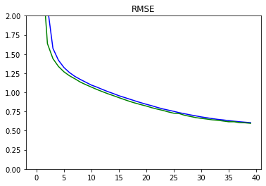
def plot_metrics(metric_name, title, ylim=5):
    plt.title(title)
    plt.ylim(0,ylim)
    plt.plot(history.history[metric_name],color='blue',label=metric_name)
    plt.plot(history.history['val_' + metric_name],color='green',label='val_' + metric_name)

def plot_confusion_matrix(y_true, y_pred, title='', labels=[0,1]):
    cm = confusion_matrix(test_Y[1], np.round(type_pred), labels=[0, 1])
    disp = ConfusionMatrixDisplay(confusion_matrix=cm,
                                  display_labels=[0, 1])
    disp.plot(values_format='d');

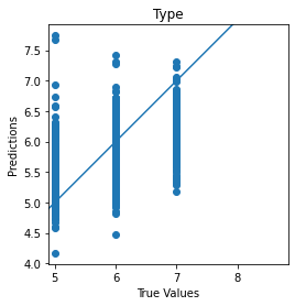
def plot_diff(y_true, y_pred, title = '' ):
    plt.scatter(y_true, y_pred)
    plt.title(title)
    plt.xlabel('True Values')
    plt.ylabel('Predictions')
    plt.axis('equal')
    plt.axis('square')
    plt.plot([-100, 100], [-100, 100])
    return plt

Plots for Metrics

plot_metrics('wine_quality_root_mean_squared_error', 'RMSE', ylim=2)

png

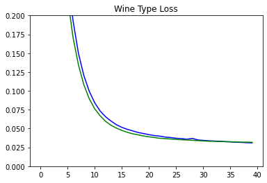
plot_metrics('wine_type_loss', 'Wine Type Loss', ylim=0.2)

png

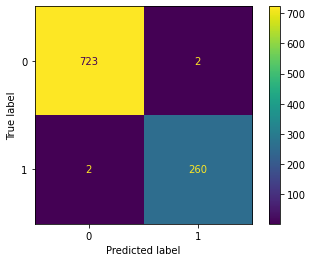
Plots for Confusion Matrix

Plot the confusion matrices for wine type. You can see that the model performs well for prediction of wine type from the confusion matrix and the loss metrics.

plot_confusion_matrix(test_Y[1], np.round(type_pred), title='Wine Type', labels = [0, 1])

png

scatter_plot = plot_diff(test_Y[0], quality_pred, title='Type')

png