Coursera

Custom Training Basics

In this ungraded lab you’ll gain a basic understanding of building custom training loops.

• It takes you through the underlying logic of fitting any model to a set of inputs and outputs.
• You will be training your model on the linear equation for a straight line, wx + b.
• You will implement basic linear regression from scratch using gradient tape.
• You will try to minimize the loss incurred by the model using linear regression.

Imports

from __future__ import absolute_import, division, print_function, unicode_literals

try:
  # %tensorflow_version only exists in Colab.
  %tensorflow_version 2.x
except Exception:
  pass


import tensorflow as tf
import numpy as np
import matplotlib.pyplot as plt

Define Model

You define your model as a class.

• x is your input tensor.
• The model should output values of wx+b.
• You’ll start off by initializing w and b to random values.
• During the training process, values of w and b get updated in accordance with linear regression so as to minimize the loss incurred by the model.
• Once you arrive at optimal values for w and b, the model would have been trained to correctly predict the values of wx+b.

Hence,

• w and b are trainable weights of the model.
• x is the input
• y = wx + b is the output

class Model(object):
  def __init__(self):
    # Initialize the weights to `2.0` and the bias to `1.0`
    # In practice, these should be initialized to random values (for example, with `tf.random.normal`)
    self.w = tf.Variable(2.0)
    self.b = tf.Variable(1.0)

  def __call__(self, x):
    return self.w * x + self.b

model = Model()

Define a loss function

A loss function measures how well the output of a model for a given input matches the target output.

• The goal is to minimize this difference during training.
• Let’s use the standard L2 loss, also known as the least square errors $$Loss = \sum_{i} \left (y_{pred}^i - y_{target}^i \right )^2$$

def loss(predicted_y, target_y):
  return tf.reduce_mean(tf.square(predicted_y - target_y))

Obtain training data

First, synthesize the training data using the “true” w and “true” b.

$$y = w_{true} \times x + b_{true} $$

TRUE_w = 3.0
TRUE_b = 2.0
NUM_EXAMPLES = 1000

xs  = tf.random.normal(shape=[NUM_EXAMPLES])

ys = (TRUE_w * xs) + TRUE_b

Before training the model, visualize the loss value by plotting the model’s predictions in red crosses and the training data in blue dots:

def plot_data(inputs, outputs, predicted_outputs):
  real = plt.scatter(inputs, outputs, c='b', marker='.')
  predicted = plt.scatter(inputs, predicted_outputs, c='r', marker='+')
  plt.legend((real,predicted), ('Real Data', 'Predicted Data'))
  plt.show()

plot_data(xs, ys, model(xs))
print('Current loss: %1.6f' % loss(model(xs), ys).numpy())

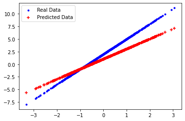
Current loss: 2.037160

Define a training loop

With the network and training data, train the model using gradient descent

• Gradient descent updates the trainable weights w and b to reduce the loss.

There are many variants of the gradient descent scheme that are captured in tf.train.Optimizer—our recommended implementation. In the spirit of building from first principles, here you will implement the basic math yourself.

• You’ll use tf.GradientTape for automatic differentiation
• Use tf.assign_sub for decrementing a value. Note that assign_sub combines tf.assign and tf.sub

def train(model, inputs, outputs, learning_rate):
  with tf.GradientTape() as t:
    current_loss = loss(model(inputs), outputs)
  dw, db = t.gradient(current_loss, [model.w, model.b])
  model.w.assign_sub(learning_rate * dw)
  model.b.assign_sub(learning_rate * db)

  return current_loss

Finally, you can iteratively run through the training data and see how w and b evolve.

model = Model()

# Collect the history of W-values and b-values to plot later
list_w, list_b = [], []
epochs = range(15)
losses = []
for epoch in epochs:
  list_w.append(model.w.numpy())
  list_b.append(model.b.numpy())
  current_loss = train(model, xs, ys, learning_rate=0.1)
  losses.append(current_loss)
  print('Epoch %2d: w=%1.2f b=%1.2f, loss=%2.5f' %
        (epoch, list_w[-1], list_b[-1], current_loss))

Epoch  0: w=2.00 b=1.00, loss=2.03716
Epoch  1: w=2.20 b=1.20, loss=1.29169
Epoch  2: w=2.37 b=1.36, loss=0.81902
Epoch  3: w=2.50 b=1.49, loss=0.51931
Epoch  4: w=2.60 b=1.60, loss=0.32928
Epoch  5: w=2.68 b=1.68, loss=0.20879
Epoch  6: w=2.75 b=1.74, loss=0.13239
Epoch  7: w=2.80 b=1.80, loss=0.08394
Epoch  8: w=2.84 b=1.84, loss=0.05323
Epoch  9: w=2.87 b=1.87, loss=0.03375
Epoch 10: w=2.90 b=1.90, loss=0.02140
Epoch 11: w=2.92 b=1.92, loss=0.01357
Epoch 12: w=2.94 b=1.93, loss=0.00860
Epoch 13: w=2.95 b=1.95, loss=0.00546
Epoch 14: w=2.96 b=1.96, loss=0.00346

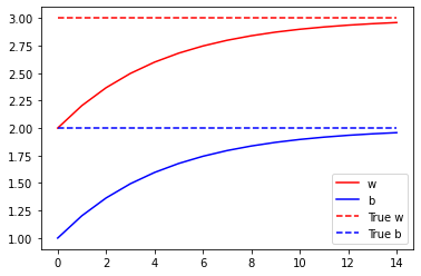
In addition to the values for losses, you also plot the progression of trainable variables over epochs.

plt.plot(epochs, list_w, 'r',
       epochs, list_b, 'b')
plt.plot([TRUE_w] * len(epochs), 'r--',
      [TRUE_b] * len(epochs), 'b--')
plt.legend(['w', 'b', 'True w', 'True b'])
plt.show()

Plots for Evaluation

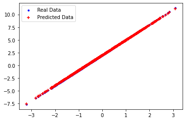
Now you can plot the actual outputs in red and the model’s predictions in blue on a set of random test examples.

You can see that the model is able to make predictions on the test set fairly accurately.

test_inputs  = tf.random.normal(shape=[NUM_EXAMPLES])
test_outputs = test_inputs * TRUE_w + TRUE_b

predicted_test_outputs = model(test_inputs)
plot_data(test_inputs, test_outputs, predicted_test_outputs)

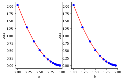
Visualize the cost function against the values of each of the trainable weights the model approximated to over time.

def plot_loss_for_weights(weights_list, losses):
  for idx, weights in enumerate(weights_list):
    plt.subplot(120 + idx + 1)
    plt.plot(weights['values'], losses, 'r')
    plt.plot(weights['values'], losses, 'bo')
    plt.xlabel(weights['name'])
    plt.ylabel('Loss')
    
    
weights_list = [{ 'name' : "w",
                  'values' : list_w
                },
                {
                  'name' : "b",
                  'values' : list_b
                }]

plot_loss_for_weights(weights_list, losses)