Coursera
Breast Cancer Prediction
In this exercise, you will train a neural network on the Breast Cancer Dataset to predict if the tumor is malignant or benign.
If you get stuck, we recommend that you review the ungraded labs for this week.
Imports
import tensorflow as tf
from tensorflow.keras.models import Model
from tensorflow.keras.layers import Dense, Input

import numpy as np
import matplotlib.pyplot as plt
import matplotlib.ticker as mticker
import pandas as pd
from sklearn.model_selection import train_test_split
from sklearn.metrics import confusion_matrix
import itertools
from tqdm import tqdm
import tensorflow_datasets as tfds

tf.get_logger().setLevel('ERROR')
Load and Preprocess the Dataset
We first load the dataset and create a data frame using pandas. We explicitly specify the column names because the CSV file does not have column headers.
data_file = './data/data.csv'
col_names = ["id", "clump_thickness", "un_cell_size", "un_cell_shape", "marginal_adheshion", "single_eph_cell_size", "bare_nuclei", "bland_chromatin", "normal_nucleoli", "mitoses", "class"]
df = pd.read_csv(data_file, names=col_names, header=None)
df.head()
.dataframe tbody tr th {
    vertical-align: top;
}

.dataframe thead th {
    text-align: right;
}
| id | clump_thickness | un_cell_size | un_cell_shape | marginal_adheshion | single_eph_cell_size | bare_nuclei | bland_chromatin | normal_nucleoli | mitoses | class | |
|---|---|---|---|---|---|---|---|---|---|---|---|
| 0 | 1000025 | 5 | 1 | 1 | 1 | 2 | 1 | 3 | 1 | 1 | 2 |
| 1 | 1002945 | 5 | 4 | 4 | 5 | 7 | 10 | 3 | 2 | 1 | 2 |
| 2 | 1015425 | 3 | 1 | 1 | 1 | 2 | 2 | 3 | 1 | 1 | 2 |
| 3 | 1016277 | 6 | 8 | 8 | 1 | 3 | 4 | 3 | 7 | 1 | 2 |
| 4 | 1017023 | 4 | 1 | 1 | 3 | 2 | 1 | 3 | 1 | 1 | 2 |
We have to do some preprocessing on the data. We first pop the id column since it is of no use for our problem at hand.
df.pop("id")
0      1000025
1      1002945
2      1015425
3      1016277
4      1017023
        ...
694     776715
695     841769
696     888820
697     897471
698     897471
Name: id, Length: 699, dtype: int64
Upon inspection of data, you can see that some values of the bare_nuclei column are unknown. We drop the rows with these unknown values. We also convert the bare_nuclei column to numeric. This is required for training the model.
df = df[df["bare_nuclei"] != '?' ]
df.bare_nuclei = pd.to_numeric(df.bare_nuclei)
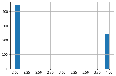
We check the class distribution of the data. You can see that there are two classes, 2.0 and 4.0 According to the dataset:
- 2.0 = benign
- 4.0 = malignant
df['class'].hist(bins=20)
<matplotlib.axes._subplots.AxesSubplot at 0x7f9d149abe10>
We are going to model this problem as a binary classification problem which detects whether the tumor is malignant or not. Hence, we change the dataset so that:
- benign(2.0) = 0
- malignant(4.0) = 1
df['class'] = np.where(df['class'] == 2, 0, 1)
We then split the dataset into training and testing sets. Since the number of samples is small, we will perform validation on the test set.
train, test = train_test_split(df, test_size = 0.2)
We get the statistics for training. We can look at statistics to get an idea about the distribution of plots. If you need more visualization, you can create additional data plots. We will also be using the mean and standard deviation from statistics for normalizing the data
train_stats = train.describe()
train_stats.pop('class')
train_stats = train_stats.transpose()
We pop the class column from the training and test sets to create train and test outputs.
train_Y = train.pop("class")
test_Y = test.pop("class")
Here we normalize the data by using the formula: X = (X - mean(X)) / StandardDeviation(X)
def norm(x):
    return (x - train_stats['mean']) / train_stats['std']
norm_train_X = norm(train)
norm_test_X = norm(test)
We now create Tensorflow datasets for training and test sets to easily be able to build and manage an input pipeline for our model.
train_dataset = tf.data.Dataset.from_tensor_slices((norm_train_X.values, train_Y.values))
test_dataset = tf.data.Dataset.from_tensor_slices((norm_test_X.values, test_Y.values))
We shuffle and prepare a batched dataset to be used for training in our custom training loop.
batch_size = 32
train_dataset = train_dataset.shuffle(buffer_size=len(train)).batch(batch_size)

test_dataset =  test_dataset.batch(batch_size=batch_size)
a = enumerate(train_dataset)

print(len(list(a)))
18
Define the Model
Now we will define the model. Here, we use the Keras Functional API to create a simple network of two Dense layers. We have modelled the problem as a binary classification problem and hence we add a single layer with sigmoid activation as the final layer of the model.
def base_model():
    inputs = tf.keras.layers.Input(shape=(len(train.columns)))

    x = tf.keras.layers.Dense(128, activation='relu')(inputs)
    x = tf.keras.layers.Dense(64, activation='relu')(x)
    outputs = tf.keras.layers.Dense(1, activation='sigmoid')(x)
    model = tf.keras.Model(inputs=inputs, outputs=outputs)
    return model

model = base_model()
Define Optimizer and Loss
We use RMSprop optimizer and binary crossentropy as our loss function.
optimizer = tf.keras.optimizers.RMSprop(learning_rate=0.001)
loss_object = tf.keras.losses.BinaryCrossentropy()
Evaluate Untrained Model
We calculate the loss on the model before training begins.
outputs = model(norm_test_X.values)
loss_value = loss_object(y_true=test_Y.values, y_pred=outputs)
print("Loss before training %.4f" % loss_value.numpy())
Loss before training 0.7011
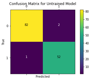
We also plot the confusion matrix to visualize the true outputs against the outputs predicted by the model.
def plot_confusion_matrix(y_true, y_pred, title='', labels=[0,1]):
    cm = confusion_matrix(y_true, y_pred)
    fig = plt.figure()
    ax = fig.add_subplot(111)
    cax = ax.matshow(cm)
    plt.title(title)
    fig.colorbar(cax)
    ax.set_xticklabels([''] + labels)
    ax.set_yticklabels([''] + labels)
    plt.xlabel('Predicted')
    plt.ylabel('True')
    fmt = 'd'
    thresh = cm.max() / 2.
    for i, j in itertools.product(range(cm.shape[0]), range(cm.shape[1])):
          plt.text(j, i, format(cm[i, j], fmt),
                  horizontalalignment="center",
                  color="black" if cm[i, j] > thresh else "white")
    plt.show()
plot_confusion_matrix(test_Y.values, tf.round(outputs), title='Confusion Matrix for Untrained Model')
Define Metrics (Please complete this section)
Define Custom F1Score Metric
In this example, we will define a custom F1Score metric using the formula.
F1 Score = 2 * ((precision * recall) / (precision + recall))
precision = true_positives / (true_positives + false_positives)
recall = true_positives / (true_positives + false_negatives)
We use confusion_matrix defined in tf.math to calculate precision and recall.
Here you can see that we have subclassed tf.keras.Metric and implemented the three required methods update_state, result and reset_states.
Please complete the result() method:
class F1Score(tf.keras.metrics.Metric):

    def __init__(self, name='f1_score', **kwargs):
        '''initializes attributes of the class'''

        # call the parent class init
        super(F1Score, self).__init__(name=name, **kwargs)

        # Initialize Required variables
        # true positives
        self.tp = tf.Variable(0, dtype = 'int32')
        # false positives
        self.fp = tf.Variable(0, dtype = 'int32')
        # true negatives
        self.tn = tf.Variable(0, dtype = 'int32')
        # false negatives
        self.fn = tf.Variable(0, dtype = 'int32')

    def update_state(self, y_true, y_pred, sample_weight=None):
        '''
        Accumulates statistics for the metric

        Args:
            y_true: target values from the test data
            y_pred: predicted values by the model
        '''

        # Calulcate confusion matrix.
        conf_matrix = tf.math.confusion_matrix(y_true, y_pred, num_classes=2)

        # Update values of true positives, true negatives, false positives and false negatives from confusion matrix.
        self.tn.assign_add(conf_matrix[0][0])
        self.tp.assign_add(conf_matrix[1][1])
        self.fp.assign_add(conf_matrix[0][1])
        self.fn.assign_add(conf_matrix[1][0])

    def result(self):
        '''Computes and returns the metric value tensor.'''

        # Calculate precision
        if (self.tp + self.fp == 0):
            precision = 1.0
        else:
            precision = self.tp / (self.tp + self.fp)

        # Calculate recall
        if (self.tp + self.fn == 0):
            recall = 1.0
        else:
            recall = self.tp / (self.tp + self.fn)

        # Return F1 Score
        ### START CODE HERE ###
        f1_score = 2 * ((precision * recall) / (precision + recall))
        ### END CODE HERE ###

        return f1_score

    def reset_states(self):
        '''Resets all of the metric state variables.'''

        # The state of the metric will be reset at the start of each epoch.
        self.tp.assign(0)
        self.tn.assign(0)
        self.fp.assign(0)
        self.fn.assign(0)
# Test Code:

test_F1Score = F1Score()

test_F1Score.tp = tf.Variable(2, dtype = 'int32')
test_F1Score.fp = tf.Variable(5, dtype = 'int32')
test_F1Score.tn = tf.Variable(7, dtype = 'int32')
test_F1Score.fn = tf.Variable(9, dtype = 'int32')
test_F1Score.result()
<tf.Tensor: shape=(), dtype=float64, numpy=0.2222222222222222>
Expected Output:
><tf.Tensor: shape=(), dtype=float64, numpy=0.2222222222222222>
We initialize the seprate metrics required for training and validation. In addition to our custom F1Score metric, we are also using BinaryAccuracy defined in tf.keras.metrics
train_f1score_metric = F1Score()
val_f1score_metric = F1Score()

train_acc_metric = tf.keras.metrics.BinaryAccuracy()
val_acc_metric = tf.keras.metrics.BinaryAccuracy()
Apply Gradients (Please complete this section)
The core of training is using the model to calculate the logits on specific set of inputs and compute the loss(in this case binary crossentropy) by comparing the predicted outputs to the true outputs. We then update the trainable weights using the optimizer algorithm chosen. The optimizer algorithm requires our computed loss and partial derivatives of loss with respect to each of the trainable weights to make updates to the same.
We use gradient tape to calculate the gradients and then update the model trainable weights using the optimizer.
Please complete the following function:
def apply_gradient(optimizer, loss_object, model, x, y):
    '''
    applies the gradients to the trainable model weights

    Args:
        optimizer: optimizer to update model weights
        loss_object: type of loss to measure during training
        model: the model we are training
        x: input data to the model
        y: target values for each input
    '''

    with tf.GradientTape() as tape:
    ### START CODE HERE ###
        logits = model(x)
        loss_value = loss_object(y_true=y, y_pred=logits)

    gradients = tape.gradient(loss_value, model.trainable_weights)
    optimizer.apply_gradients(zip(gradients, model.trainable_weights))
    ### END CODE HERE ###

    return logits, loss_value
# Test Code:

test_model = tf.keras.models.load_model('./test_model')
test_logits, test_loss = apply_gradient(optimizer, loss_object, test_model, norm_test_X.values, test_Y.values)

print(test_logits.numpy()[:8])
print(test_loss.numpy())

del test_model
del test_logits
del test_loss
[[0.5234933 ]
 [0.45760757]
 [0.44932652]
 [0.5293622 ]
 [0.51498365]
 [0.53253335]
 [0.5353688 ]
 [0.52803123]]
0.7056353
Expected Output:
The output will be close to these values:
>[[0.5516499 ]
 [0.52124363]
 [0.5412698 ]
 [0.54203206]
 [0.50022954]
 [0.5459626 ]
 [0.47841492]
 [0.54381996]]
0.7030578
Training Loop (Please complete this section)
This function performs training during one epoch. We run through all batches of training data in each epoch to make updates to trainable weights using our previous function.
You can see that we also call update_state on our metrics to accumulate the value of our metrics.
We are displaying a progress bar to indicate completion of training in each epoch. Here we use tqdm for displaying the progress bar.
Please complete the following function:
def train_data_for_one_epoch(train_dataset, optimizer, loss_object, model,
                             train_acc_metric, train_f1score_metric, verbose=True):
    '''
    Computes the loss then updates the weights and metrics for one epoch.

    Args:
        train_dataset: the training dataset
        optimizer: optimizer to update model weights
        loss_object: type of loss to measure during training
        model: the model we are training
        train_acc_metric: calculates how often predictions match labels
        train_f1score_metric: custom metric we defined earlier
    '''
    losses = []

    #Iterate through all batches of training data
    for step, (x_batch_train, y_batch_train) in enumerate(train_dataset):

        #Calculate loss and update trainable variables using optimizer
        ### START CODE HERE ###
        logits, loss_value = apply_gradient(optimizer=optimizer,
                                            loss_object=loss_object,
                                            model=model,
                                            x=x_batch_train,
                                            y=y_batch_train)
        losses.append(loss_value)
        ### END CODE HERE ###

        #Round off logits to nearest integer and cast to integer for calulating metrics
        logits = tf.round(logits)
        logits = tf.cast(logits, 'int64')

        #Update the training metrics
        ### START CODE HERE ###
        train_acc_metric.update_state(y_batch_train, logits)
        train_f1score_metric.update_state(y_batch_train, logits)
        ### END CODE HERE ###

        #Update progress
        if verbose:
            print("Training loss for step %s: %.4f" % (int(step), float(loss_value)))

    return losses
# TEST CODE

test_model = tf.keras.models.load_model('./test_model')

test_losses = train_data_for_one_epoch(train_dataset, optimizer, loss_object, test_model,
                             train_acc_metric, train_f1score_metric, verbose=False)

for test_loss in test_losses:
    print(test_loss.numpy())

del test_model
del test_losses
0.75029516
0.59677184
0.55122435
0.4755624
0.42687407
0.44664067
0.4167109
0.34282595
0.2860944
0.33811605
0.29171586
0.33543205
0.2677728
0.28945237
0.31126976
0.22086957
0.24056101
0.10725332
Expected Output:
The losses should generally be decreasing and will start from around 0.75. For example:
0.7600615
0.6092045
0.5525634
0.4358902
0.4765755
0.43327087
0.40585428
0.32855004
0.35755336
0.3651728
0.33971977
0.27372319
0.25026917
0.29229593
0.242178
0.20602849
0.15887335
0.090397514
At the end of each epoch, we have to validate the model on the test dataset. The following function calculates the loss on test dataset and updates the states of the validation metrics.
def perform_validation():
    losses = []

    #Iterate through all batches of validation data.
    for x_val, y_val in test_dataset:

        #Calculate validation loss for current batch.
        val_logits = model(x_val)
        val_loss = loss_object(y_true=y_val, y_pred=val_logits)
        losses.append(val_loss)

        #Round off and cast outputs to either  or 1
        val_logits = tf.cast(tf.round(model(x_val)), 'int64')

        #Update validation metrics
        val_acc_metric.update_state(y_val, val_logits)
        val_f1score_metric.update_state(y_val, val_logits)

    return losses
Next we define the training loop that runs through the training samples repeatedly over a fixed number of epochs. Here we combine the functions we built earlier to establish the following flow:
- Perform training over all batches of training data.
- Get values of metrics.
- Perform validation to calculate loss and update validation metrics on test data.
- Reset the metrics at the end of epoch.
- Display statistics at the end of each epoch.
Note : We also calculate the training and validation losses for the whole epoch at the end of the epoch.
# Iterate over epochs.
epochs = 5
epochs_val_losses, epochs_train_losses = [], []

for epoch in range(epochs):
    print('Start of epoch %d' % (epoch,))
    #Perform Training over all batches of train data
    losses_train = train_data_for_one_epoch(train_dataset, optimizer, loss_object, model, train_acc_metric, train_f1score_metric)

    # Get results from training metrics
    train_acc = train_acc_metric.result()
    train_f1score = train_f1score_metric.result()

    #Perform validation on all batches of test data
    losses_val = perform_validation()

    # Get results from validation metrics
    val_acc = val_acc_metric.result()
    val_f1score = val_f1score_metric.result()

    #Calculate training and validation losses for current epoch
    losses_train_mean = np.mean(losses_train)
    losses_val_mean = np.mean(losses_val)
    epochs_val_losses.append(losses_val_mean)
    epochs_train_losses.append(losses_train_mean)

    print('\n Epcoh %s: Train loss: %.4f  Validation Loss: %.4f, Train Accuracy: %.4f, Validation Accuracy %.4f, Train F1 Score: %.4f, Validation F1 Score: %.4f' % (epoch, float(losses_train_mean), float(losses_val_mean), float(train_acc), float(val_acc), train_f1score, val_f1score))

    #Reset states of all metrics
    train_acc_metric.reset_states()
    val_acc_metric.reset_states()
    val_f1score_metric.reset_states()
    train_f1score_metric.reset_states()
Start of epoch 0
Training loss for step 0: 0.6753
Training loss for step 1: 0.5670
Training loss for step 2: 0.4764
Training loss for step 3: 0.4131
Training loss for step 4: 0.3930
Training loss for step 5: 0.3557
Training loss for step 6: 0.2707
Training loss for step 7: 0.2977
Training loss for step 8: 0.2479
Training loss for step 9: 0.2556
Training loss for step 10: 0.2287
Training loss for step 11: 0.1681
Training loss for step 12: 0.1974
Training loss for step 13: 0.1663
Training loss for step 14: 0.1329
Training loss for step 15: 0.1750
Training loss for step 16: 0.1920
Training loss for step 17: 0.0503

 Epcoh 0: Train loss: 0.2924  Validation Loss: 0.1372, Train Accuracy: 0.9314, Validation Accuracy 0.9750, Train F1 Score: 0.8983, Validation F1 Score: 0.9630
Start of epoch 1
Training loss for step 0: 0.1317
Training loss for step 1: 0.1217
Training loss for step 2: 0.1196
Training loss for step 3: 0.1718
Training loss for step 4: 0.1532
Training loss for step 5: 0.0529
Training loss for step 6: 0.2426
Training loss for step 7: 0.0686
Training loss for step 8: 0.0479
Training loss for step 9: 0.1115
Training loss for step 10: 0.0477
Training loss for step 11: 0.0637
Training loss for step 12: 0.1196
Training loss for step 13: 0.0881
Training loss for step 14: 0.1000
Training loss for step 15: 0.0488
Training loss for step 16: 0.1710
Training loss for step 17: 0.5051

 Epcoh 1: Train loss: 0.1314  Validation Loss: 0.0813, Train Accuracy: 0.9427, Validation Accuracy 0.9812, Train F1 Score: 0.9521, Validation F1 Score: 0.9720
Start of epoch 2
Training loss for step 0: 0.0364
Training loss for step 1: 0.0866
Training loss for step 2: 0.0385
Training loss for step 3: 0.0814
Training loss for step 4: 0.0354
Training loss for step 5: 0.1812
Training loss for step 6: 0.0781
Training loss for step 7: 0.1867
Training loss for step 8: 0.0312
Training loss for step 9: 0.0243
Training loss for step 10: 0.1113
Training loss for step 11: 0.0605
Training loss for step 12: 0.0396
Training loss for step 13: 0.1907
Training loss for step 14: 0.1355
Training loss for step 15: 0.0450
Training loss for step 16: 0.0559
Training loss for step 17: 0.0036

 Epcoh 2: Train loss: 0.0790  Validation Loss: 0.0667, Train Accuracy: 0.9705, Validation Accuracy 0.9812, Train F1 Score: 0.9547, Validation F1 Score: 0.9720
Start of epoch 3
Training loss for step 0: 0.0510
Training loss for step 1: 0.0575
Training loss for step 2: 0.0535
Training loss for step 3: 0.0174
Training loss for step 4: 0.0411
Training loss for step 5: 0.1278
Training loss for step 6: 0.0456
Training loss for step 7: 0.2031
Training loss for step 8: 0.1029
Training loss for step 9: 0.1386
Training loss for step 10: 0.0517
Training loss for step 11: 0.1437
Training loss for step 12: 0.0334
Training loss for step 13: 0.1147
Training loss for step 14: 0.0272
Training loss for step 15: 0.0439
Training loss for step 16: 0.0157
Training loss for step 17: 0.0209

 Epcoh 3: Train loss: 0.0716  Validation Loss: 0.0608, Train Accuracy: 0.9705, Validation Accuracy 0.9812, Train F1 Score: 0.9547, Validation F1 Score: 0.9720
Start of epoch 4
Training loss for step 0: 0.0371
Training loss for step 1: 0.1190
Training loss for step 2: 0.0149
Training loss for step 3: 0.0155
Training loss for step 4: 0.1925
Training loss for step 5: 0.1056
Training loss for step 6: 0.0130
Training loss for step 7: 0.0190
Training loss for step 8: 0.0119
Training loss for step 9: 0.1222
Training loss for step 10: 0.0625
Training loss for step 11: 0.0678
Training loss for step 12: 0.1001
Training loss for step 13: 0.0339
Training loss for step 14: 0.0948
Training loss for step 15: 0.1284
Training loss for step 16: 0.0492
Training loss for step 17: 0.0189

 Epcoh 4: Train loss: 0.0670  Validation Loss: 0.0580, Train Accuracy: 0.9740, Validation Accuracy 0.9812, Train F1 Score: 0.9600, Validation F1 Score: 0.9720
Evaluate the Model
Plots for Evaluation
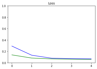
We plot the progress of loss as training proceeds over number of epochs.
def plot_metrics(train_metric, val_metric, metric_name, title, ylim=5):
    plt.title(title)
    plt.ylim(0,ylim)
    plt.gca().xaxis.set_major_locator(mticker.MultipleLocator(1))
    plt.plot(train_metric,color='blue',label=metric_name)
    plt.plot(val_metric,color='green',label='val_' + metric_name)

plot_metrics(epochs_train_losses, epochs_val_losses, "Loss", "Loss", ylim=1.0)
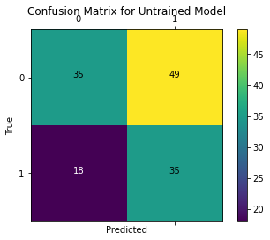
We plot the confusion matrix to visualize the true values against the values predicted by the model.
test_outputs = model(norm_test_X.values)
plot_confusion_matrix(test_Y.values, tf.round(test_outputs), title='Confusion Matrix for Untrained Model')