Coursera
Ungraded Lab: GradCAM
This lab will walk you through generating gradient-weighted class activation maps (GradCAMs) for model predictions.
- This is similar to the CAMs you generated before except:
- GradCAMs uses gradients instead of the global average pooling weights to weight the activations.
Imports
%tensorflow_version 2.x

import warnings
warnings.filterwarnings("ignore")

import os
import glob
import cv2
from pathlib import Path

import numpy as np
import pandas as pd
import matplotlib.pyplot as plt
import seaborn as sns

from skimage.io import imread, imsave
from skimage.transform import resize
from sklearn.model_selection import train_test_split
from tensorflow.keras.models import Model
from tensorflow.keras import layers
from tensorflow.keras.applications import vgg16
from tensorflow.keras.utils import to_categorical
from tensorflow.keras.optimizers import SGD, Adam, RMSprop

import tensorflow as tf
import tensorflow.keras.backend as K
import tensorflow_datasets as tfds
import tensorflow_hub as hub

import imgaug as ia
from imgaug import augmenters as iaa
Colab only includes TensorFlow 2.x; %tensorflow_version has no effect.
Download and Prepare the Dataset
You will use the Cats vs Dogs dataset again for this exercise. The following will prepare the train, test, and eval sets.
tfds.disable_progress_bar()

splits = ['train[:80%]', 'train[80%:90%]', 'train[90%:]']

# load the dataset given the splits defined above
splits, info = tfds.load('cats_vs_dogs', with_info=True, as_supervised=True, split = splits)

(train_examples, validation_examples, test_examples) = splits

num_examples = info.splits['train'].num_examples
num_classes = info.features['label'].num_classes
Downloading and preparing dataset 786.68 MiB (download: 786.68 MiB, generated: Unknown size, total: 786.68 MiB) to /root/tensorflow_datasets/cats_vs_dogs/4.0.0...


WARNING:absl:1738 images were corrupted and were skipped


Dataset cats_vs_dogs downloaded and prepared to /root/tensorflow_datasets/cats_vs_dogs/4.0.0. Subsequent calls will reuse this data.
BATCH_SIZE = 32
IMAGE_SIZE = (224, 224)

# resizes the image and normalizes the pixel values
def format_image(image, label):
  image = tf.image.resize(image, IMAGE_SIZE) / 255.0
  return  image, label

# prepare batches
train_batches = train_examples.shuffle(num_examples // 4).map(format_image).batch(BATCH_SIZE).prefetch(tf.data.experimental.AUTOTUNE)
validation_batches = validation_examples.map(format_image).batch(BATCH_SIZE).prefetch(tf.data.experimental.AUTOTUNE)
test_batches = test_examples.map(format_image).batch(1)
Modelling
You will use a pre-trained VGG16 network as your base model for the classifier. This will be followed by a global average pooling (GAP) and a 2-neuron Dense layer with softmax activation for the output. The earlier VGG blocks will be frozen and we will just fine-tune the final layers during training. These steps are shown in the utility function below.
def build_model():
  # load the base VGG16 model
  base_model = vgg16.VGG16(input_shape=IMAGE_SIZE + (3,),
                      weights='imagenet',
                      include_top=False)

  # add a GAP layer
  output = layers.GlobalAveragePooling2D()(base_model.output)

  # output has two neurons for the 2 classes (cats and dogs)
  output = layers.Dense(2, activation='softmax')(output)

  # set the inputs and outputs of the model
  model = Model(base_model.input, output)

  # freeze the earlier layers
  for layer in base_model.layers[:-4]:
      layer.trainable=False

  # choose the optimizer
  optimizer = tf.keras.optimizers.RMSprop(0.001)

  # configure the model for training
  model.compile(loss='sparse_categorical_crossentropy',
                optimizer=optimizer,
                metrics=['accuracy'])

  # display the summary
  model.summary()

  return model
model = build_model()
Downloading data from https://storage.googleapis.com/tensorflow/keras-applications/vgg16/vgg16_weights_tf_dim_ordering_tf_kernels_notop.h5
58889256/58889256 [==============================] - 1s 0us/step
Model: "model"
_________________________________________________________________
 Layer (type)                Output Shape              Param #
=================================================================
 input_1 (InputLayer)        [(None, 224, 224, 3)]     0

 block1_conv1 (Conv2D)       (None, 224, 224, 64)      1792

 block1_conv2 (Conv2D)       (None, 224, 224, 64)      36928

 block1_pool (MaxPooling2D)  (None, 112, 112, 64)      0

 block2_conv1 (Conv2D)       (None, 112, 112, 128)     73856

 block2_conv2 (Conv2D)       (None, 112, 112, 128)     147584

 block2_pool (MaxPooling2D)  (None, 56, 56, 128)       0

 block3_conv1 (Conv2D)       (None, 56, 56, 256)       295168

 block3_conv2 (Conv2D)       (None, 56, 56, 256)       590080

 block3_conv3 (Conv2D)       (None, 56, 56, 256)       590080

 block3_pool (MaxPooling2D)  (None, 28, 28, 256)       0

 block4_conv1 (Conv2D)       (None, 28, 28, 512)       1180160

 block4_conv2 (Conv2D)       (None, 28, 28, 512)       2359808

 block4_conv3 (Conv2D)       (None, 28, 28, 512)       2359808

 block4_pool (MaxPooling2D)  (None, 14, 14, 512)       0

 block5_conv1 (Conv2D)       (None, 14, 14, 512)       2359808

 block5_conv2 (Conv2D)       (None, 14, 14, 512)       2359808

 block5_conv3 (Conv2D)       (None, 14, 14, 512)       2359808

 block5_pool (MaxPooling2D)  (None, 7, 7, 512)         0

 global_average_pooling2d (  (None, 512)               0
 GlobalAveragePooling2D)

 dense (Dense)               (None, 2)                 1026

=================================================================
Total params: 14715714 (56.14 MB)
Trainable params: 7080450 (27.01 MB)
Non-trainable params: 7635264 (29.13 MB)
_________________________________________________________________
You can now train the model. This will take around 10 minutes to run.
EPOCHS = 3
model.fit(train_batches,
          epochs=EPOCHS,
          validation_data=validation_batches)
Epoch 1/3
582/582 [==============================] - 131s 190ms/step - loss: 0.7971 - accuracy: 0.8023 - val_loss: 0.1512 - val_accuracy: 0.9351
Epoch 2/3
582/582 [==============================] - 102s 166ms/step - loss: 0.1417 - accuracy: 0.9471 - val_loss: 0.1115 - val_accuracy: 0.9561
Epoch 3/3
582/582 [==============================] - 103s 166ms/step - loss: 0.0949 - accuracy: 0.9658 - val_loss: 0.1108 - val_accuracy: 0.9604


<keras.src.callbacks.History at 0x7adca9c05210>
Model Interpretability
Let’s now go through the steps to generate the class activation maps. You will start by specifying the layers you want to visualize.
# select all the layers for which you want to visualize the outputs and store it in a list
outputs = [layer.output for layer in model.layers[1:18]]

# Define a new model that generates the above output
vis_model = Model(model.input, outputs)

# store the layer names we are interested in
layer_names = []
for layer in outputs:
    layer_names.append(layer.name.split("/")[0])


print("Layers that will be used for visualization: ")
print(layer_names)
Layers that will be used for visualization:
['block1_conv1', 'block1_conv2', 'block1_pool', 'block2_conv1', 'block2_conv2', 'block2_pool', 'block3_conv1', 'block3_conv2', 'block3_conv3', 'block3_pool', 'block4_conv1', 'block4_conv2', 'block4_conv3', 'block4_pool', 'block5_conv1', 'block5_conv2', 'block5_conv3']
Class activation maps (GradCAM)
We’ll define a few more functions to output the maps. get_CAM() is the function highlighted in the lectures and takes care of generating the heatmap of gradient weighted features. show_random_sample() takes care of plotting the results.
def get_CAM(processed_image, actual_label, layer_name='block5_conv3'):
    model_grad = Model([model.inputs],
                       [model.get_layer(layer_name).output, model.output])

    with tf.GradientTape() as tape:
        conv_output_values, predictions = model_grad(processed_image)

        # watch the conv_output_values
        tape.watch(conv_output_values)

        ## Use binary cross entropy loss
        ## actual_label is 0 if cat, 1 if dog
        # get prediction probability of dog
        # If model does well,
        # pred_prob should be close to 0 if cat, close to 1 if dog
        pred_prob = predictions[:,1]

        # make sure actual_label is a float, like the rest of the loss calculation
        actual_label = tf.cast(actual_label, dtype=tf.float32)

        # add a tiny value to avoid log of 0
        smoothing = 0.00001

        # Calculate loss as binary cross entropy
        loss = -1 * (actual_label * tf.math.log(pred_prob + smoothing) + (1 - actual_label) * tf.math.log(1 - pred_prob + smoothing))
        print(f"binary loss: {loss}")

    # get the gradient of the loss with respect to the outputs of the last conv layer
    grads_values = tape.gradient(loss, conv_output_values)
    grads_values = K.mean(grads_values, axis=(0,1,2))

    conv_output_values = np.squeeze(conv_output_values.numpy())
    grads_values = grads_values.numpy()

    # weight the convolution outputs with the computed gradients
    for i in range(512):
        conv_output_values[:,:,i] *= grads_values[i]
    heatmap = np.mean(conv_output_values, axis=-1)

    heatmap = np.maximum(heatmap, 0)
    heatmap /= heatmap.max()

    del model_grad, conv_output_values, grads_values, loss

    return heatmap
def show_sample(idx=None):
# if image index is specified, get that image
if idx:
for img, label in test_batches.take(idx):
sample_image = img[0]
sample_label = label[0]
# otherwise if idx is not specified, get a random image
else:
for img, label in test_batches.shuffle(1000).take(1):
sample_image = img[0]
sample_label = label[0]
sample_image_processed = np.expand_dims(sample_image, axis=0)
activations = vis_model.predict(sample_image_processed)
pred_label = np.argmax(model.predict(sample_image_processed), axis=-1)[0]
sample_activation = activations[0][0,:,:,16]
sample_activation-=sample_activation.mean()
sample_activation/=sample_activation.std()
sample_activation *=255
sample_activation = np.clip(sample_activation, 0, 255).astype(np.uint8)
heatmap = get_CAM(sample_image_processed, sample_label)
heatmap = cv2.resize(heatmap, (sample_image.shape[0], sample_image.shape[1]))
heatmap = heatmap *255
heatmap = np.clip(heatmap, 0, 255).astype(np.uint8)
heatmap = cv2.applyColorMap(heatmap, cv2.COLORMAP_HOT)
converted_img = sample_image.numpy()
super_imposed_image = cv2.addWeighted(converted_img, 0.8, heatmap.astype('float32'), 2e-3, 0.0)
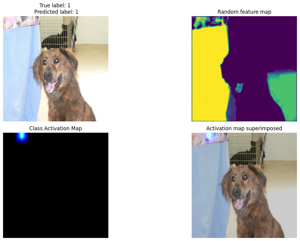
f,ax = plt.subplots(2,2, figsize=(15,8))
ax[0,0].imshow(sample_image)
ax[0,0].set_title(f"True label: {sample_label} \n Predicted label: {pred_label}")
ax[0,0].axis('off')
ax[0,1].imshow(sample_activation)
ax[0,1].set_title("Random feature map")
ax[0,1].axis('off')
ax[1,0].imshow(heatmap)
ax[1,0].set_title("Class Activation Map")
ax[1,0].axis('off')
ax[1,1].imshow(super_imposed_image)
ax[1,1].set_title("Activation map superimposed")
ax[1,1].axis('off')
plt.tight_layout()
plt.show()
return activations
Time to visualize the results
# Choose an image index to show, or leave it as None to get a random image
activations = show_sample(idx=None)
1/1 [==============================] - 1s 797ms/step
1/1 [==============================] - 0s 164ms/step
binary loss: [-1.001353e-05]


WARNING:matplotlib.image:Clipping input data to the valid range for imshow with RGB data ([0..1] for floats or [0..255] for integers).
Intermediate activations of layers
You can use the utility function below to visualize the activations in the intermediate layers you defined earlier. This plots the feature side by side for each convolution layer starting from the earliest layer all the way to the final convolution layer.
def visualize_intermediate_activations(layer_names, activations):
    assert len(layer_names)==len(activations), "Make sure layers and activation values match"
    images_per_row=16

    for layer_name, layer_activation in zip(layer_names, activations):
        nb_features = layer_activation.shape[-1]
        size= layer_activation.shape[1]

        nb_cols = nb_features // images_per_row
        grid = np.zeros((size*nb_cols, size*images_per_row))

        for col in range(nb_cols):
            for row in range(images_per_row):
                feature_map = layer_activation[0,:,:,col*images_per_row + row]
                feature_map -= feature_map.mean()
                feature_map /= feature_map.std()
                feature_map *=255
                feature_map = np.clip(feature_map, 0, 255).astype(np.uint8)

                grid[col*size:(col+1)*size, row*size:(row+1)*size] = feature_map

        scale = 1./size
        plt.figure(figsize=(scale*grid.shape[1], scale*grid.shape[0]))
        plt.title(layer_name)
        plt.grid(False)
        plt.axis('off')
        plt.imshow(grid, aspect='auto', cmap='viridis')
    plt.show()
visualize_intermediate_activations(activations=activations,
                                   layer_names=layer_names)
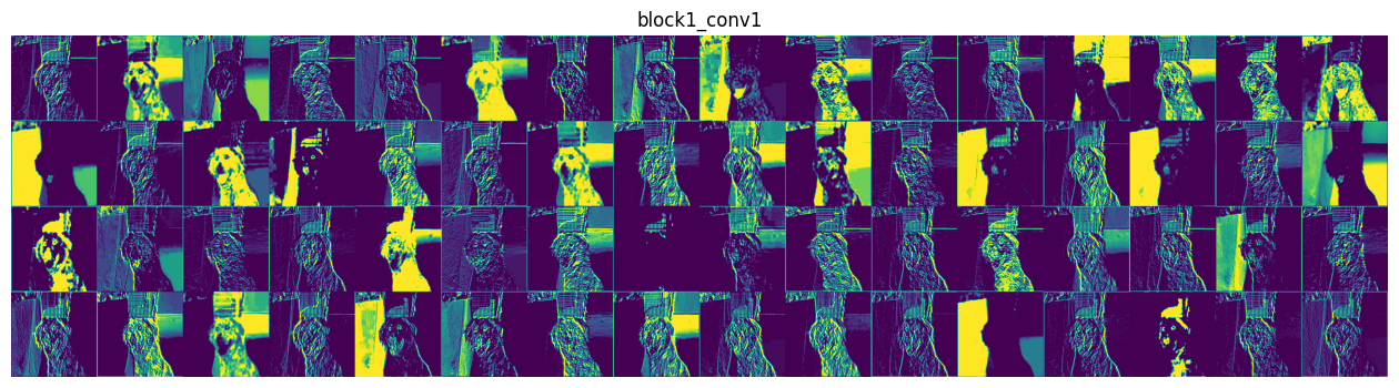
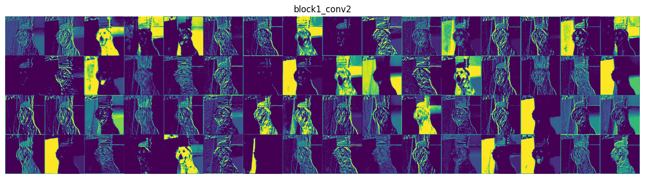
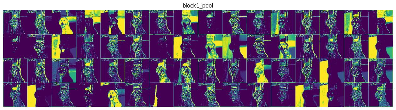
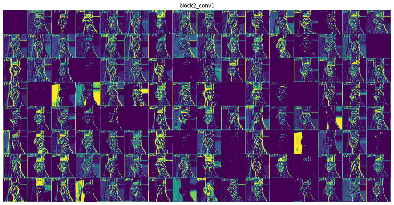
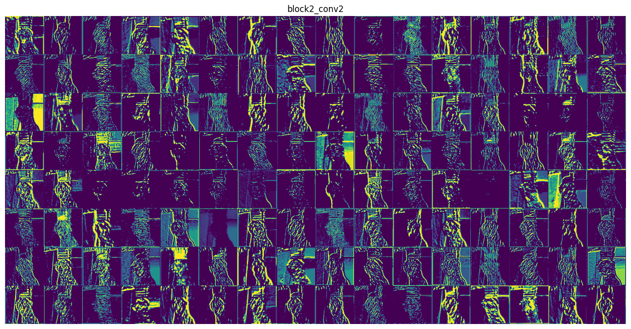
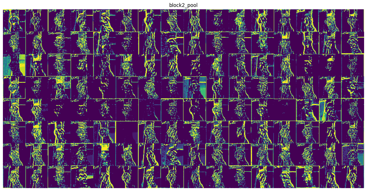
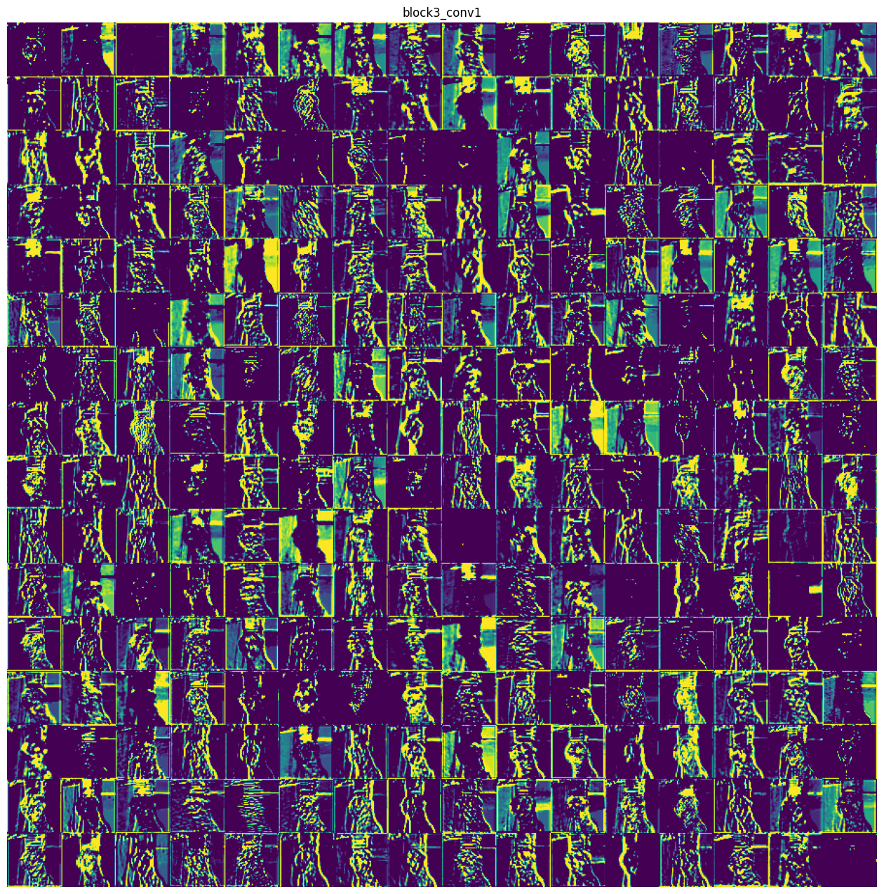
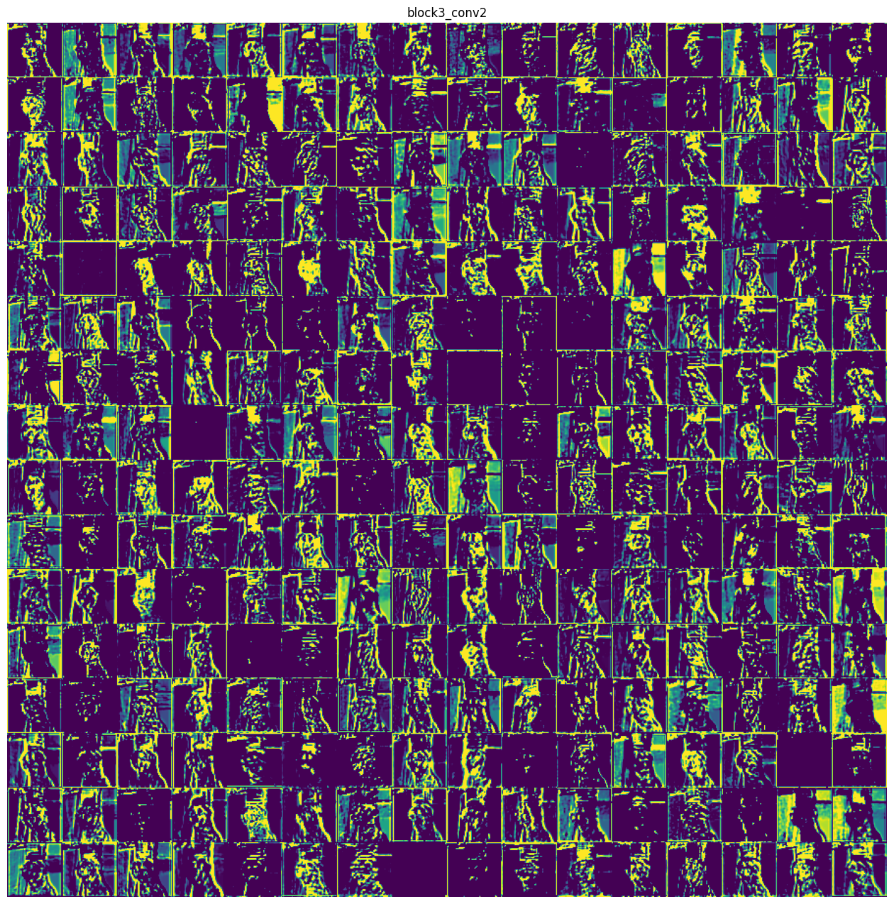
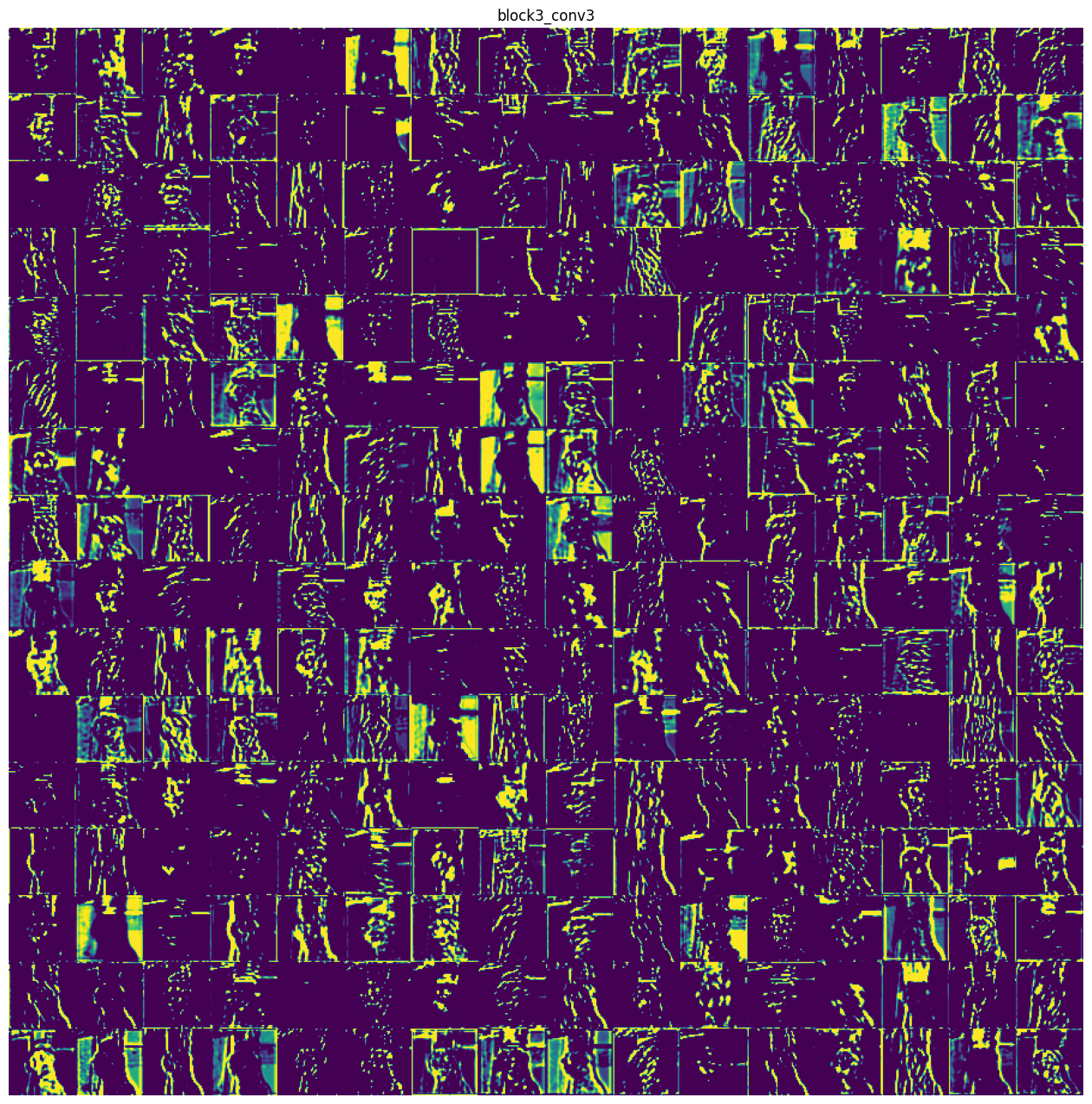
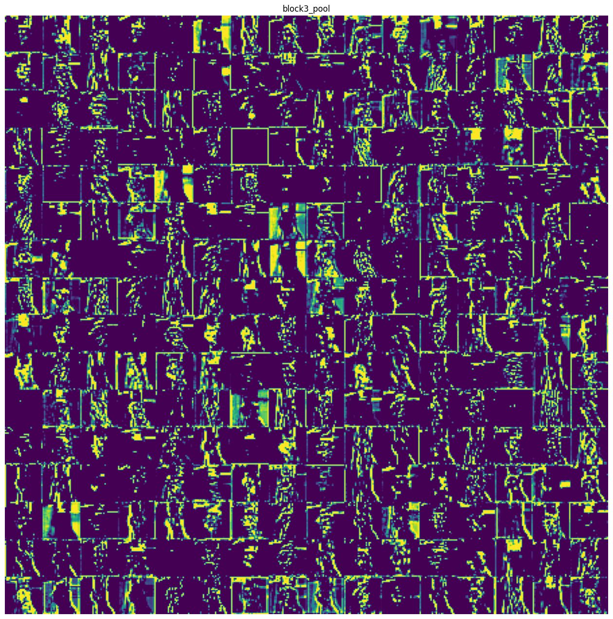
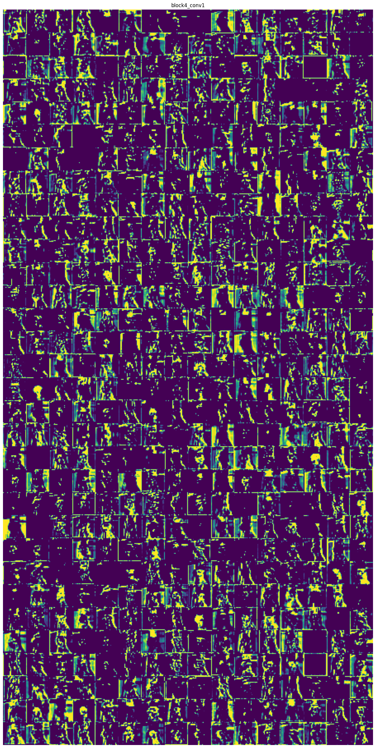
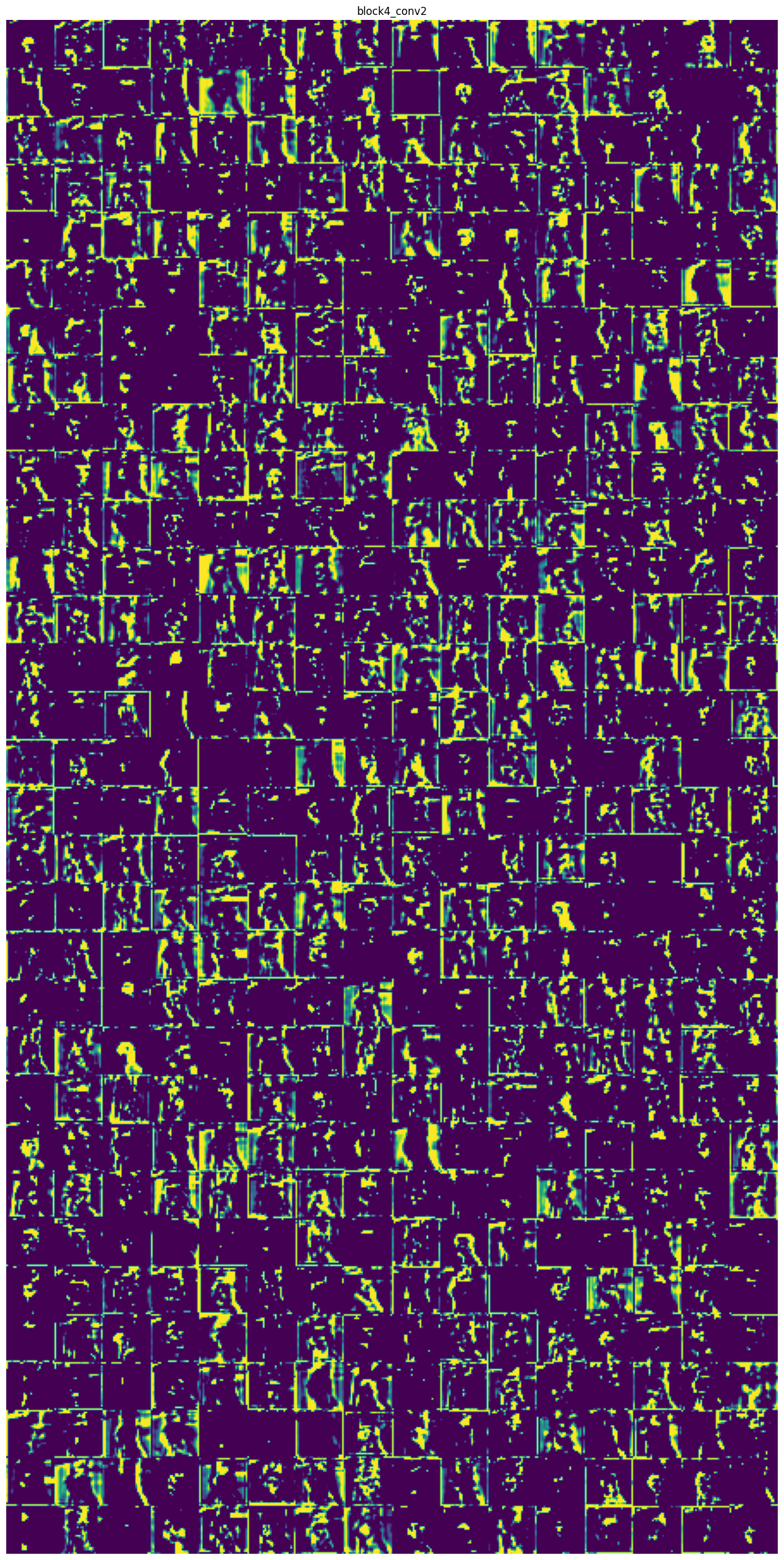
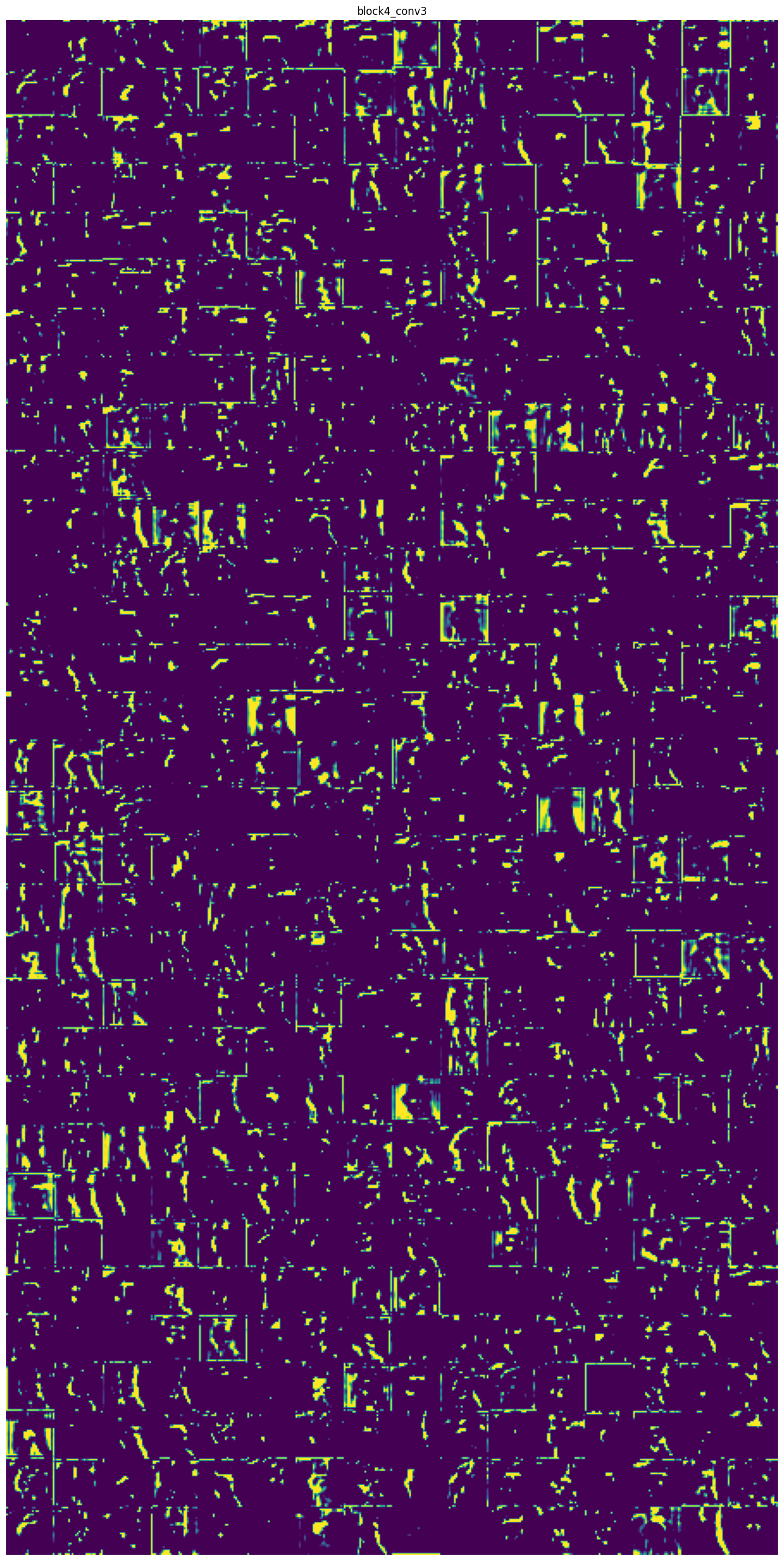
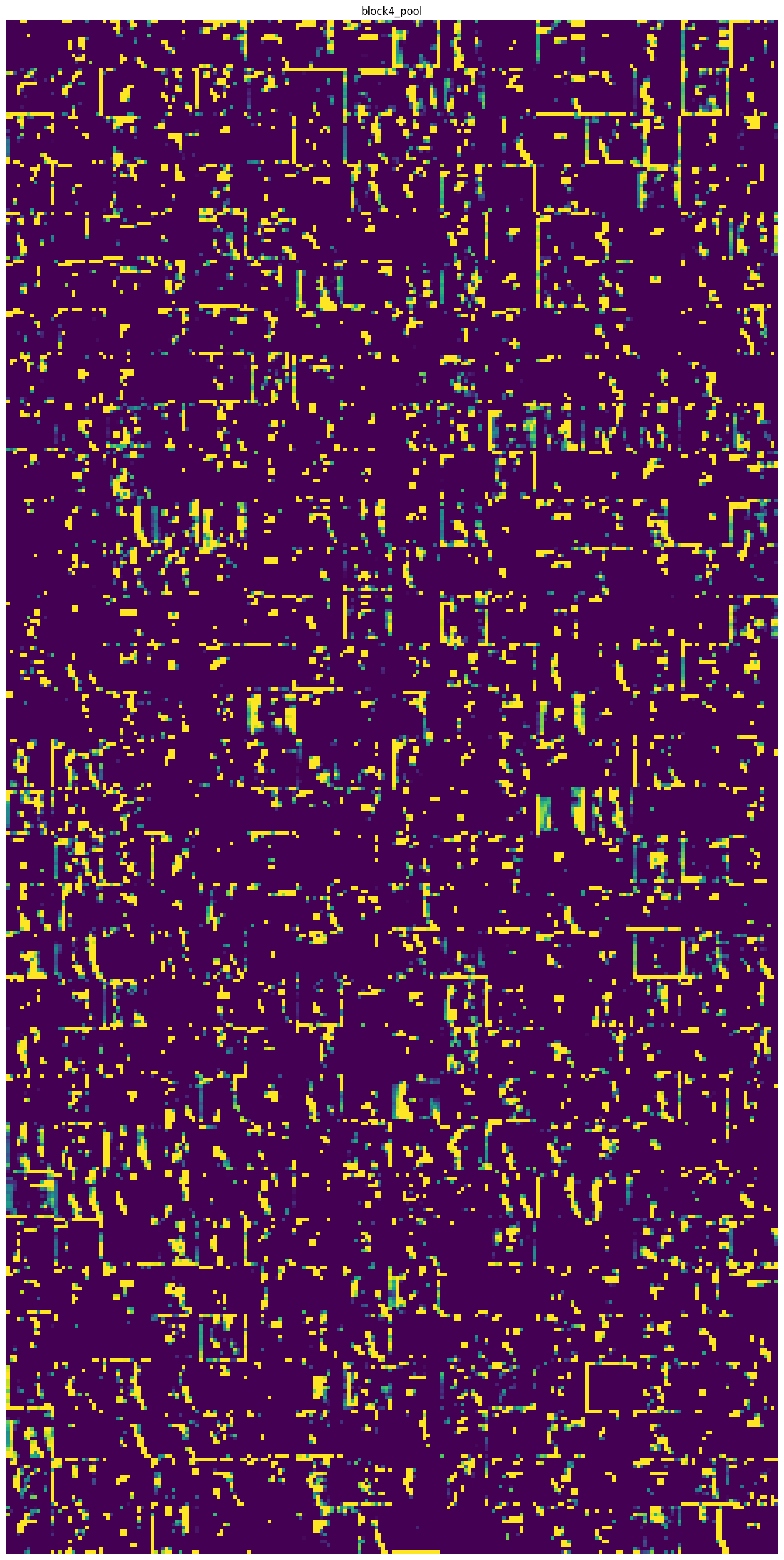
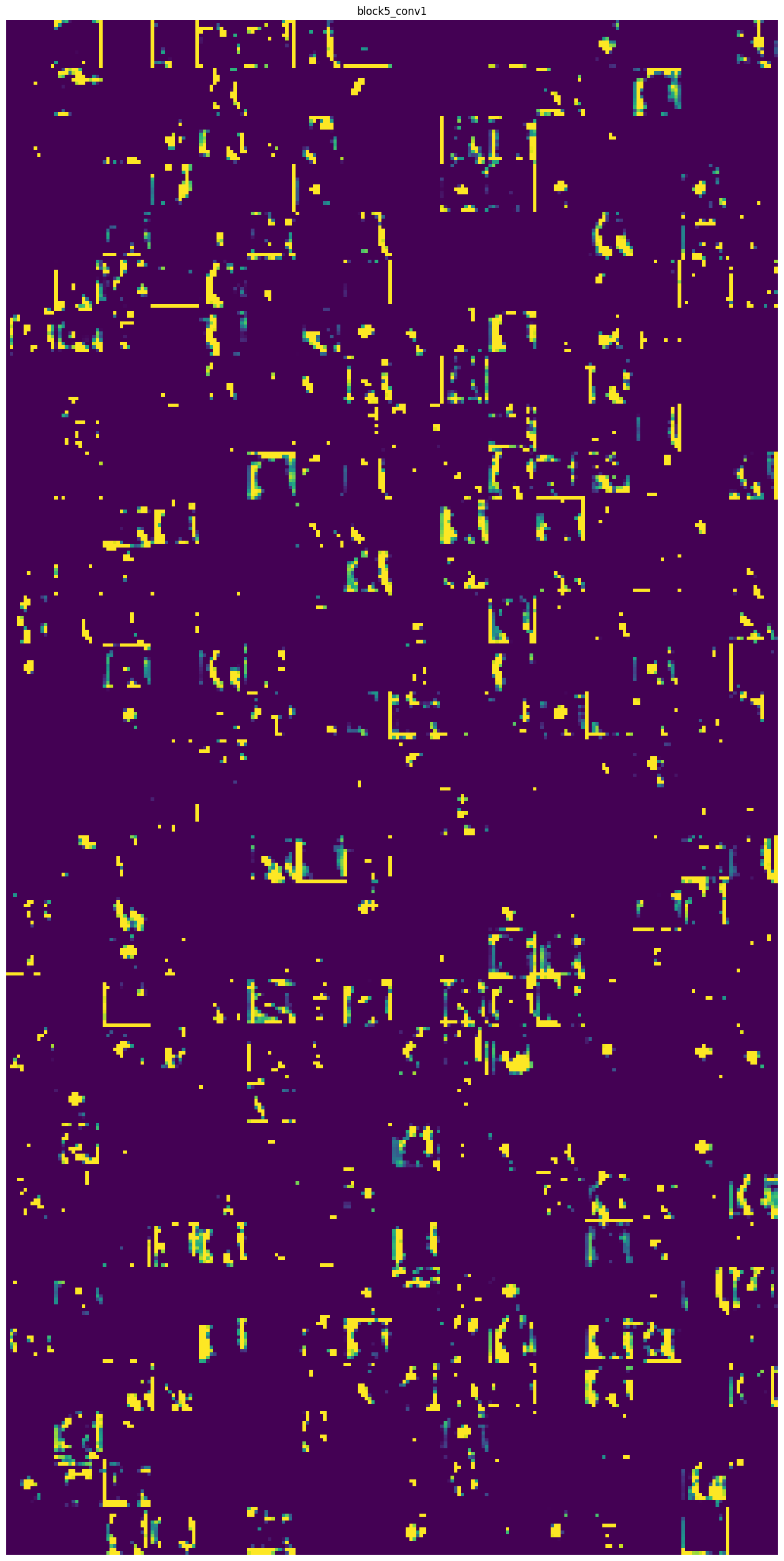
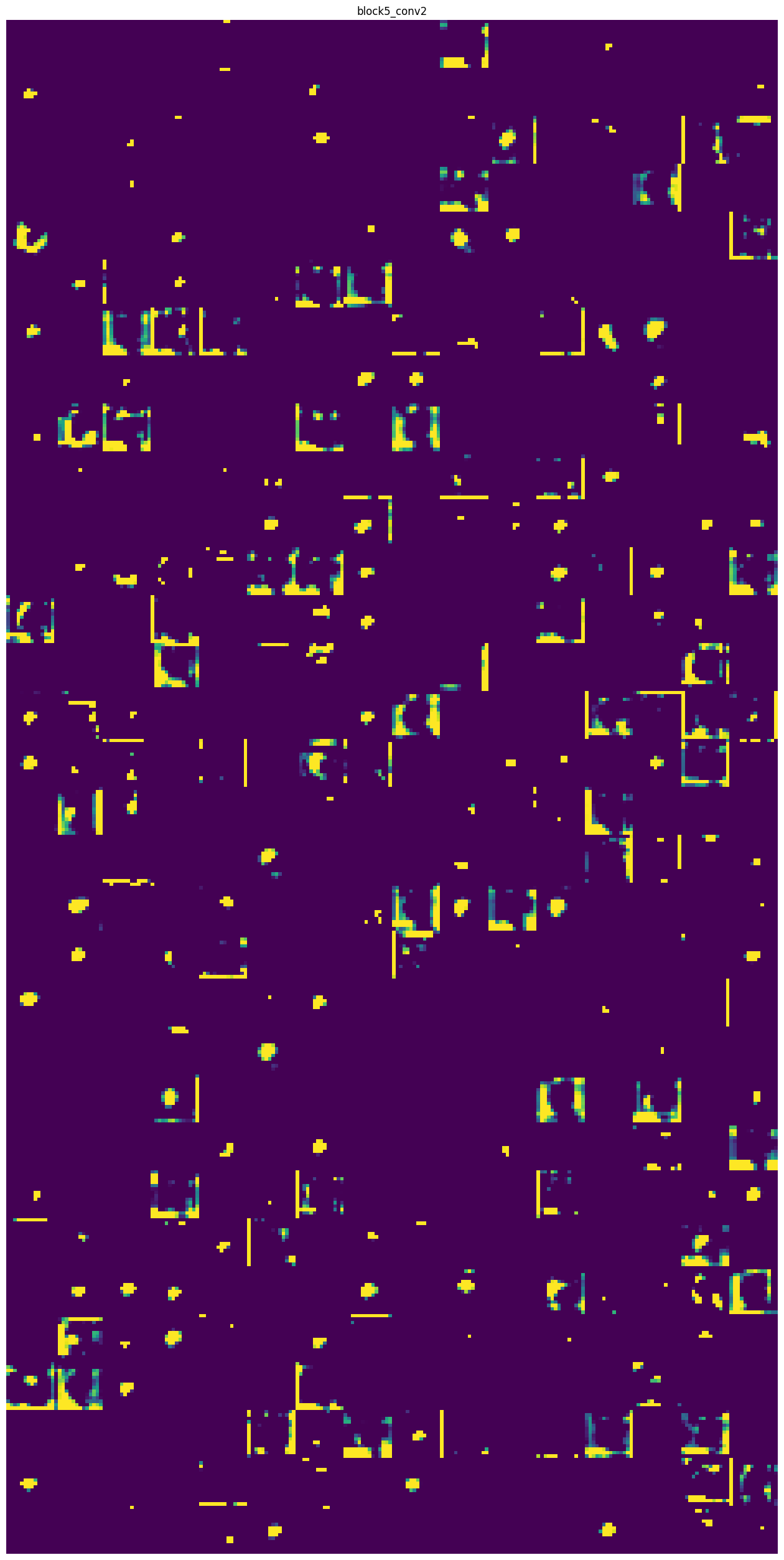
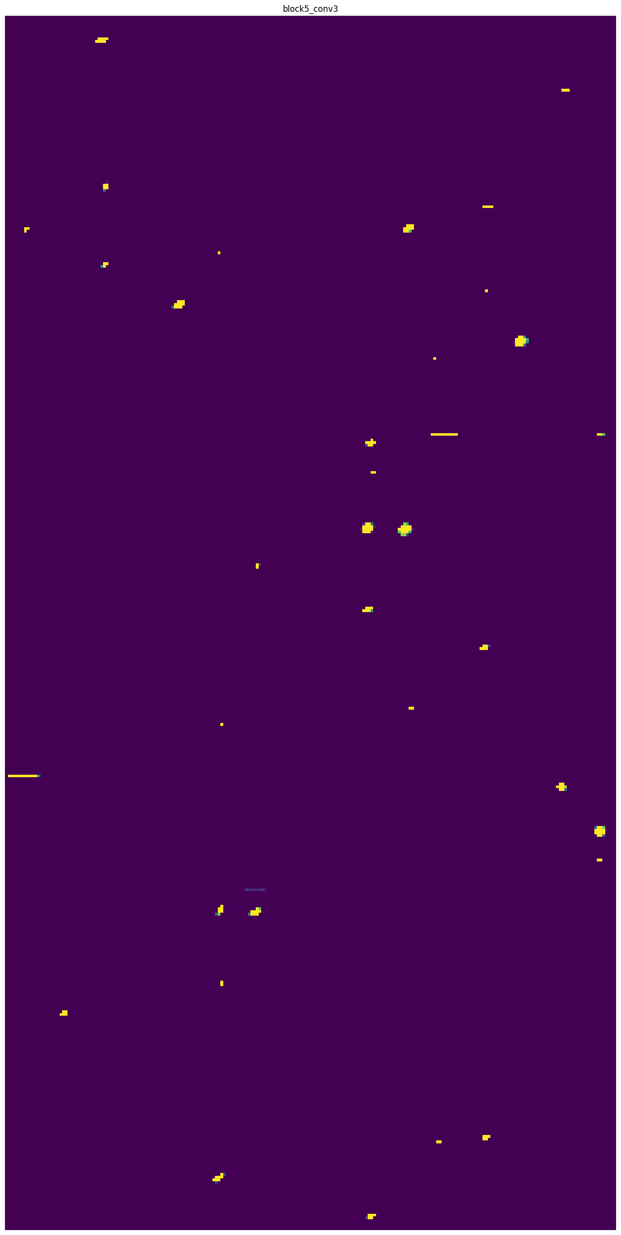
If you scroll all the way down to see the outputs of the final conv layer, you’ll see that there are very few active features and these are mostly located in the face of the cat. This is the region of the image that your model looks at when determining the class.