Coursera

Ungraded Lab: Saliency

Like class activation maps, saliency maps also tells us what parts of the image the model is focusing on when making its predictions.

The main difference is in saliency maps, we are just shown the relevant pixels instead of the learned features.
You can generate saliency maps by getting the gradient of the loss with respect to the image pixels.
This means that changes in certain pixels that strongly affect the loss will be shown brightly in your saliency map.

Let’s see how this is implemented in the following sections.

Imports

%tensorflow_version 2.x

import tensorflow as tf
import tensorflow_hub as hub
import cv2
import numpy as np
import matplotlib.pyplot as plt

Colab only includes TensorFlow 2.x; %tensorflow_version has no effect.

Build the model

For the classifier, you will use the Inception V3 model available in Tensorflow Hub. This has pre-trained weights that is able to detect 1001 classes. You can read more here.

# grab the model from Tensorflow hub and append a softmax activation
model = tf.keras.Sequential([
    hub.KerasLayer('https://tfhub.dev/google/tf2-preview/inception_v3/classification/4'),
    tf.keras.layers.Activation('softmax')
])

# build the model based on a specified batch input shape
model.build([None, 300, 300, 3])

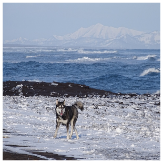
Get a sample image

You will download a photo of a Siberian Husky that our model will classify. We left the option to download a Tabby Cat image instead if you want.

!wget -O image.jpg https://cdn.pixabay.com/photo/2018/02/27/14/11/the-pacific-ocean-3185553_960_720.jpg

# If you want to try the cat, uncomment this line
# !wget -O image.jpg https://cdn.pixabay.com/photo/2018/02/27/14/11/the-pacific-ocean-3185553_960_720.jpg

--2023-10-05 02:13:28--  https://cdn.pixabay.com/photo/2018/02/27/14/11/the-pacific-ocean-3185553_960_720.jpg
Resolving cdn.pixabay.com (cdn.pixabay.com)... 172.64.147.160, 104.18.40.96, 2606:4700:4400::6812:2860, ...
Connecting to cdn.pixabay.com (cdn.pixabay.com)|172.64.147.160|:443... connected.
HTTP request sent, awaiting response... 200 OK
Length: 212830 (208K) [binary/octet-stream]
Saving to: ‘image.jpg’

image.jpg           100%[===================>] 207.84K  --.-KB/s    in 0.02s   

2023-10-05 02:13:28 (10.8 MB/s) - ‘image.jpg’ saved [212830/212830]

Preprocess the image

The image needs to be preprocessed before being fed to the model. This is done in the following steps:

# read the image
img = cv2.imread('image.jpg')

# format it to be in the RGB colorspace
img = cv2.cvtColor(img, cv2.COLOR_BGR2RGB)

# resize to 300x300 and normalize pixel values to be in the range [0, 1]
img = cv2.resize(img, (300, 300)) / 255.0

# add a batch dimension in front
image = np.expand_dims(img, axis=0)

We can now preview our input image.

plt.figure(figsize=(8, 8))
plt.imshow(img)
plt.axis('off')
plt.show()

png

Compute Gradients

You will now get the gradients of the loss with respect to the input image pixels. This is the key step to generate the map later.

# Siberian Husky's class ID in ImageNet
class_index = 251

# If you downloaded the cat, use this line instead
#class_index = 282   # Tabby Cat in ImageNet

# number of classes in the model's training data
num_classes = 1001

# convert to one hot representation to match our softmax activation in the model definition
expected_output = tf.one_hot([class_index] * image.shape[0], num_classes)

with tf.GradientTape() as tape:
    # cast image to float
    inputs = tf.cast(image, tf.float32)

    # watch the input pixels
    tape.watch(inputs)

    # generate the predictions
    predictions = model(inputs)

    # get the loss
    loss = tf.keras.losses.categorical_crossentropy(
        expected_output, predictions
    )

# get the gradient with respect to the inputs
gradients = tape.gradient(loss, inputs)

Visualize the results

Now that you have the gradients, you will do some postprocessing to generate the saliency maps and overlay it on the image.

# reduce the RGB image to grayscale
grayscale_tensor = tf.reduce_sum(tf.abs(gradients), axis=-1)

# normalize the pixel values to be in the range [0, 255].
# the max value in the grayscale tensor will be pushed to 255.
# the min value will be pushed to 0.
normalized_tensor = tf.cast(
    255
    * (grayscale_tensor - tf.reduce_min(grayscale_tensor))
    / (tf.reduce_max(grayscale_tensor) - tf.reduce_min(grayscale_tensor)),
    tf.uint8,
)

# remove the channel dimension to make the tensor a 2d tensor
normalized_tensor = tf.squeeze(normalized_tensor)

Let’s do a little sanity check to see the results of the conversion.

# max and min value in the grayscale tensor
print(np.max(grayscale_tensor[0]))
print(np.min(grayscale_tensor[0]))
print()

# coordinates of the first pixel where the max and min values are located
max_pixel = np.unravel_index(np.argmax(grayscale_tensor[0]), grayscale_tensor[0].shape)
min_pixel = np.unravel_index(np.argmin(grayscale_tensor[0]), grayscale_tensor[0].shape)
print(max_pixel)
print(min_pixel)
print()

# these coordinates should have the max (255) and min (0) value in the normalized tensor
print(normalized_tensor[max_pixel])
print(normalized_tensor[min_pixel])

1.0859327
0.0

(207, 132)
(0, 299)

tf.Tensor(255, shape=(), dtype=uint8)
tf.Tensor(0, shape=(), dtype=uint8)

You should get something like:

1.2167013
0.0

(203, 129)
(0, 299)

tf.Tensor(255, shape=(), dtype=uint8)
tf.Tensor(0, shape=(), dtype=uint8)

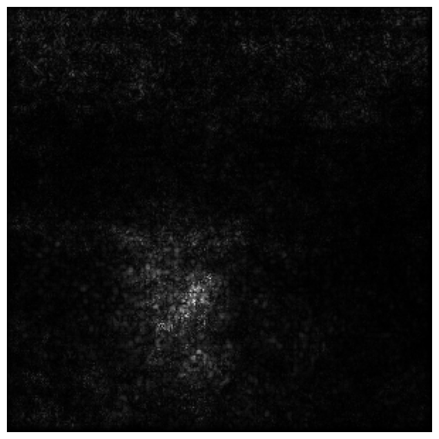
Now let’s see what this looks like when plotted. The white pixels show the parts the model focused on when classifying the image.

plt.figure(figsize=(8, 8))
plt.axis('off')
plt.imshow(normalized_tensor, cmap='gray')
plt.show()

png

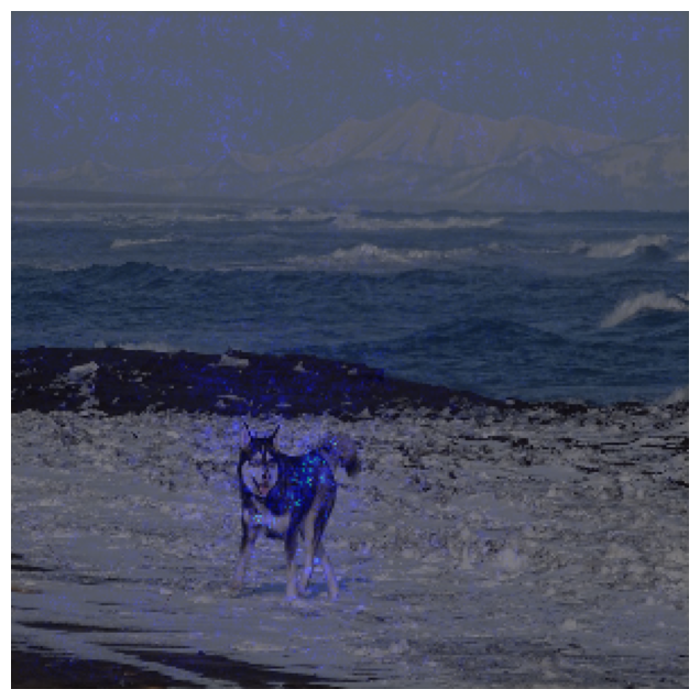
Let’s superimpose the normalized tensor to the input image to get more context. You can see that the strong pixels are over the husky and that is a good indication that the model is looking at the correct part of the image.

gradient_color = cv2.applyColorMap(normalized_tensor.numpy(), cv2.COLORMAP_HOT)
gradient_color = gradient_color / 255.0
super_imposed = cv2.addWeighted(img, 0.5, gradient_color, 0.5, 0.0)

plt.figure(figsize=(8, 8))
plt.imshow(super_imposed)
plt.axis('off')
plt.show()

png