Coursera
Image Classification and Object Localization
In this lab, you’ll build a CNN from scratch to:
- classify the main subject in an image
- localize it by drawing bounding boxes around it.
You’ll use the MNIST dataset to synthesize a custom dataset for the task:
- Place each “digit” image on a black canvas of width 75 x 75 at random locations.
- Calculate the corresponding bounding boxes for those “digits”.
The bounding box prediction can be modelled as a “regression” task, which means that the model will predict a numeric value (as opposed to a category).
Imports
import os, re, time, json
import PIL.Image, PIL.ImageFont, PIL.ImageDraw
import numpy as np
try:
  # %tensorflow_version only exists in Colab.
  %tensorflow_version 2.x
except Exception:
  pass
import tensorflow as tf
from matplotlib import pyplot as plt
import tensorflow_datasets as tfds

print("Tensorflow version " + tf.__version__)
Colab only includes TensorFlow 2.x; %tensorflow_version has no effect.
Tensorflow version 2.12.0
Visualization Utilities
These functions are used to draw bounding boxes around the digits.
#@title Plot Utilities for Bounding Boxes [RUN ME]

im_width = 75
im_height = 75
use_normalized_coordinates = True

def draw_bounding_boxes_on_image_array(image,
                                       boxes,
                                       color=[],
                                       thickness=1,
                                       display_str_list=()):
  """Draws bounding boxes on image (numpy array).
  Args:
    image: a numpy array object.
    boxes: a 2 dimensional numpy array of [N, 4]: (ymin, xmin, ymax, xmax).
           The coordinates are in normalized format between [0, 1].
    color: color to draw bounding box. Default is red.
    thickness: line thickness. Default value is 4.
    display_str_list_list: a list of strings for each bounding box.
  Raises:
    ValueError: if boxes is not a [N, 4] array
  """
  image_pil = PIL.Image.fromarray(image)
  rgbimg = PIL.Image.new("RGBA", image_pil.size)
  rgbimg.paste(image_pil)
  draw_bounding_boxes_on_image(rgbimg, boxes, color, thickness,
                               display_str_list)
  return np.array(rgbimg)


def draw_bounding_boxes_on_image(image,
                                 boxes,
                                 color=[],
                                 thickness=1,
                                 display_str_list=()):
  """Draws bounding boxes on image.
  Args:
    image: a PIL.Image object.
    boxes: a 2 dimensional numpy array of [N, 4]: (ymin, xmin, ymax, xmax).
           The coordinates are in normalized format between [0, 1].
    color: color to draw bounding box. Default is red.
    thickness: line thickness. Default value is 4.
    display_str_list: a list of strings for each bounding box.

  Raises:
    ValueError: if boxes is not a [N, 4] array
  """
  boxes_shape = boxes.shape
  if not boxes_shape:
    return
  if len(boxes_shape) != 2 or boxes_shape[1] != 4:
    raise ValueError('Input must be of size [N, 4]')
  for i in range(boxes_shape[0]):
    draw_bounding_box_on_image(image, boxes[i, 1], boxes[i, 0], boxes[i, 3],
                               boxes[i, 2], color[i], thickness, display_str_list[i])

def draw_bounding_box_on_image(image,
                               ymin,
                               xmin,
                               ymax,
                               xmax,
                               color='red',
                               thickness=1,
                               display_str=None,
                               use_normalized_coordinates=True):
  """Adds a bounding box to an image.
  Bounding box coordinates can be specified in either absolute (pixel) or
  normalized coordinates by setting the use_normalized_coordinates argument.
  Args:
    image: a PIL.Image object.
    ymin: ymin of bounding box.
    xmin: xmin of bounding box.
    ymax: ymax of bounding box.
    xmax: xmax of bounding box.
    color: color to draw bounding box. Default is red.
    thickness: line thickness. Default value is 4.
    display_str_list: string to display in box
    use_normalized_coordinates: If True (default), treat coordinates
      ymin, xmin, ymax, xmax as relative to the image.  Otherwise treat
      coordinates as absolute.
  """
  draw = PIL.ImageDraw.Draw(image)
  im_width, im_height = image.size
  if use_normalized_coordinates:
    (left, right, top, bottom) = (xmin * im_width, xmax * im_width,
                                  ymin * im_height, ymax * im_height)
  else:
    (left, right, top, bottom) = (xmin, xmax, ymin, ymax)
  draw.line([(left, top), (left, bottom), (right, bottom),
             (right, top), (left, top)], width=thickness, fill=color)
These utilities are used to visualize the data and predictions.
#@title Visualization Utilities [RUN ME]
"""
This cell contains helper functions used for visualization
and downloads only.

You can skip reading it, as there is very
little Keras or Tensorflow related code here.
"""

# Matplotlib config
plt.rc('image', cmap='gray')
plt.rc('grid', linewidth=0)
plt.rc('xtick', top=False, bottom=False, labelsize='large')
plt.rc('ytick', left=False, right=False, labelsize='large')
plt.rc('axes', facecolor='F8F8F8', titlesize="large", edgecolor='white')
plt.rc('text', color='a8151a')
plt.rc('figure', facecolor='F0F0F0')# Matplotlib fonts
MATPLOTLIB_FONT_DIR = os.path.join(os.path.dirname(plt.__file__), "mpl-data/fonts/ttf")

# pull a batch from the datasets. This code is not very nice, it gets much better in eager mode (TODO)
def dataset_to_numpy_util(training_dataset, validation_dataset, N):

  # get one batch from each: 10000 validation digits, N training digits
  batch_train_ds = training_dataset.unbatch().batch(N)

  # eager execution: loop through datasets normally
  if tf.executing_eagerly():
    for validation_digits, (validation_labels, validation_bboxes) in validation_dataset:
      validation_digits = validation_digits.numpy()
      validation_labels = validation_labels.numpy()
      validation_bboxes = validation_bboxes.numpy()
      break
    for training_digits, (training_labels, training_bboxes) in batch_train_ds:
      training_digits = training_digits.numpy()
      training_labels = training_labels.numpy()
      training_bboxes = training_bboxes.numpy()
      break

  # these were one-hot encoded in the dataset
  validation_labels = np.argmax(validation_labels, axis=1)
  training_labels = np.argmax(training_labels, axis=1)

  return (training_digits, training_labels, training_bboxes,
          validation_digits, validation_labels, validation_bboxes)

# create digits from local fonts for testing
def create_digits_from_local_fonts(n):
  font_labels = []
  img = PIL.Image.new('LA', (75*n, 75), color = (0,255)) # format 'LA': black in channel 0, alpha in channel 1
  font1 = PIL.ImageFont.truetype(os.path.join(MATPLOTLIB_FONT_DIR, 'DejaVuSansMono-Oblique.ttf'), 25)
  font2 = PIL.ImageFont.truetype(os.path.join(MATPLOTLIB_FONT_DIR, 'STIXGeneral.ttf'), 25)
  d = PIL.ImageDraw.Draw(img)
  for i in range(n):
    font_labels.append(i%10)
    d.text((7+i*75,0 if i<10 else -4), str(i%10), fill=(255,255), font=font1 if i<10 else font2)
  font_digits = np.array(img.getdata(), np.float32)[:,0] / 255.0 # black in channel 0, alpha in channel 1 (discarded)
  font_digits = np.reshape(np.stack(np.split(np.reshape(font_digits, [75, 75*n]), n, axis=1), axis=0), [n, 75*75])
  return font_digits, font_labels


# utility to display a row of digits with their predictions
def display_digits_with_boxes(digits, predictions, labels, pred_bboxes, bboxes, iou, title):

  n = 10

  indexes = np.random.choice(len(predictions), size=n)
  n_digits = digits[indexes]
  n_predictions = predictions[indexes]
  n_labels = labels[indexes]

  n_iou = []
  if len(iou) > 0:
    n_iou = iou[indexes]

  if (len(pred_bboxes) > 0):
    n_pred_bboxes = pred_bboxes[indexes,:]

  if (len(bboxes) > 0):
    n_bboxes = bboxes[indexes,:]


  n_digits = n_digits * 255.0
  n_digits = n_digits.reshape(n, 75, 75)
  fig = plt.figure(figsize=(20, 4))
  plt.title(title)
  plt.yticks([])
  plt.xticks([])

  for i in range(10):
    ax = fig.add_subplot(1, 10, i+1)
    bboxes_to_plot = []
    if (len(pred_bboxes) > i):
      bboxes_to_plot.append(n_pred_bboxes[i])

    if (len(bboxes) > i):
      bboxes_to_plot.append(n_bboxes[i])

    img_to_draw = draw_bounding_boxes_on_image_array(image=n_digits[i], boxes=np.asarray(bboxes_to_plot), color=['red', 'green'], display_str_list=["true", "pred"])
    plt.xlabel(n_predictions[i])
    plt.xticks([])
    plt.yticks([])

    if n_predictions[i] != n_labels[i]:
      ax.xaxis.label.set_color('red')


    plt.imshow(img_to_draw)

    if len(iou) > i :
      color = "black"
      if (n_iou[i][0] < iou_threshold):
        color = "red"
      ax.text(0.2, -0.3, "iou: %s" %(n_iou[i][0]), color=color, transform=ax.transAxes)


# utility to display training and validation curves
def plot_metrics(metric_name, title, ylim=5):
  plt.title(title)
  plt.ylim(0,ylim)
  plt.plot(history.history[metric_name],color='blue',label=metric_name)
  plt.plot(history.history['val_' + metric_name],color='green',label='val_' + metric_name)
Selecting Between Strategies
TPU or GPU detection
Depending on the hardware available, you’ll use different distribution strategies. For a review on distribution strategies, please check out the second course in this specialization “Custom and Distributed Training with TensorFlow”, week 4, “Distributed Training”.
- If the TPU is available, then you’ll be using the TPU Strategy. Otherwise:
- If more than one GPU is available, then you’ll use the Mirrored Strategy
- If one GPU is available or if just the CPU is available, you’ll use the default strategy.
# Detect hardware
try:
  tpu = tf.distribute.cluster_resolver.TPUClusterResolver() # TPU detection
except ValueError:
  tpu = None
  gpus = tf.config.experimental.list_logical_devices("GPU")

# Select appropriate distribution strategy
if tpu:
  tf.config.experimental_connect_to_cluster(tpu)
  tf.tpu.experimental.initialize_tpu_system(tpu)
  strategy = tf.distribute.experimental.TPUStrategy(tpu) # Going back and forth between TPU and host is expensive. Better to run 128 batches on the TPU before reporting back.
  print('Running on TPU ', tpu.cluster_spec().as_dict()['worker'])
elif len(gpus) > 1:
  strategy = tf.distribute.MirroredStrategy([gpu.name for gpu in gpus])
  print('Running on multiple GPUs ', [gpu.name for gpu in gpus])
elif len(gpus) == 1:
  strategy = tf.distribute.get_strategy() # default strategy that works on CPU and single GPU
  print('Running on single GPU ', gpus[0].name)
else:
  strategy = tf.distribute.get_strategy() # default strategy that works on CPU and single GPU
  print('Running on CPU')
print("Number of accelerators: ", strategy.num_replicas_in_sync)
WARNING:absl:`tf.distribute.experimental.TPUStrategy` is deprecated, please use  the non experimental symbol `tf.distribute.TPUStrategy` instead.


Running on TPU  ['10.4.144.106:8470']
Number of accelerators:  8
Parameters
The global batch size is the batch size per replica (64 in this case) times the number of replicas in the distribution strategy.
BATCH_SIZE = 64 * strategy.num_replicas_in_sync # Gobal batch size.
# The global batch size will be automatically sharded across all
# replicas by the tf.data.Dataset API. A single TPU has 8 cores.
# The best practice is to scale the batch size by the number of
# replicas (cores). The learning rate should be increased as well.
Loading and Preprocessing the Dataset
Define some helper functions that will pre-process your data:
read_image_tfds: randomly overlays the “digit” image on top of a larger canvas.get_training_dataset: loads data and splits it to get the training set.get_validation_dataset: loads and splits the data to get the validation set.
'''
Transforms each image in dataset by pasting it on a 75x75 canvas at random locations.
'''
def read_image_tfds(image, label):
    xmin = tf.random.uniform((), 0 , 48, dtype=tf.int32)
    ymin = tf.random.uniform((), 0 , 48, dtype=tf.int32)
    image = tf.reshape(image, (28,28,1,))
    image = tf.image.pad_to_bounding_box(image, ymin, xmin, 75, 75)
    image = tf.cast(image, tf.float32)/255.0
    xmin = tf.cast(xmin, tf.float32)
    ymin = tf.cast(ymin, tf.float32)

    xmax = (xmin + 28) / 75
    ymax = (ymin + 28) / 75
    xmin = xmin / 75
    ymin = ymin / 75
    return image, (tf.one_hot(label, 10), [xmin, ymin, xmax, ymax])

'''
Loads and maps the training split of the dataset using the map function. Note that we try to load the gcs version since TPU can only work with datasets on Google Cloud Storage.
'''
def get_training_dataset():

      with  strategy.scope():
        dataset = tfds.load("mnist", split="train", as_supervised=True, try_gcs=True)
        dataset = dataset.map(read_image_tfds, num_parallel_calls=16)
        dataset = dataset.shuffle(5000, reshuffle_each_iteration=True)
        dataset = dataset.repeat() # Mandatory for Keras for now
        dataset = dataset.batch(BATCH_SIZE, drop_remainder=True) # drop_remainder is important on TPU, batch size must be fixed
        dataset = dataset.prefetch(-1)  # fetch next batches while training on the current one (-1: autotune prefetch buffer size)
      return dataset

'''
Loads and maps the validation split of the dataset using the map function. Note that we try to load the gcs version since TPU can only work with datasets on Google Cloud Storage.
'''
def get_validation_dataset():
    dataset = tfds.load("mnist", split="test", as_supervised=True, try_gcs=True)
    dataset = dataset.map(read_image_tfds, num_parallel_calls=16)

    #dataset = dataset.cache() # this small dataset can be entirely cached in RAM
    dataset = dataset.batch(10000, drop_remainder=True) # 10000 items in eval dataset, all in one batch
    dataset = dataset.repeat() # Mandatory for Keras for now
    return dataset

# instantiate the datasets
with strategy.scope():
  training_dataset = get_training_dataset()
  validation_dataset = get_validation_dataset()
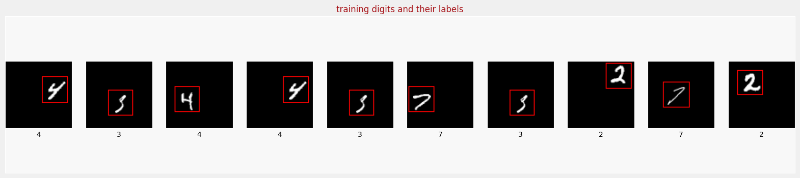
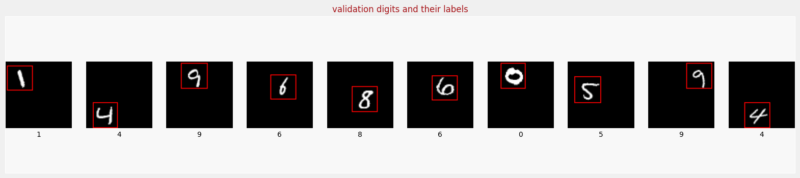
Visualize Data
(training_digits, training_labels, training_bboxes,
 validation_digits, validation_labels, validation_bboxes) = dataset_to_numpy_util(training_dataset, validation_dataset, 10)

display_digits_with_boxes(training_digits, training_labels, training_labels, np.array([]), training_bboxes, np.array([]), "training digits and their labels")
display_digits_with_boxes(validation_digits, validation_labels, validation_labels, np.array([]), validation_bboxes, np.array([]), "validation digits and their labels")
Define the Network
Here, you’ll define your custom CNN.
feature_extractor: these convolutional layers extract the features of the image.classifier: This define the output layer that predicts among 10 categories (digits 0 through 9)bounding_box_regression: This defines the output layer that predicts 4 numeric values, which define the coordinates of the bounding box (xmin, ymin, xmax, ymax)final_model: This combines the layers for feature extraction, classification and bounding box prediction.- Notice that this is another example of a branching model, because the model splits to produce two kinds of output (a category and set of numbers).
- Since you’ve learned to use the Functional API earlier in the specialization (course 1), you have the flexibility to define this kind of branching model!
define_and_compile_model: choose the optimizer and metrics, then compile the model.
'''
Feature extractor is the CNN that is made up of convolution and pooling layers.
'''
def feature_extractor(inputs):
    x = tf.keras.layers.Conv2D(16, activation='relu', kernel_size=3, input_shape=(75, 75, 1))(inputs)
    x = tf.keras.layers.AveragePooling2D((2, 2))(x)

    x = tf.keras.layers.Conv2D(32,kernel_size=3,activation='relu')(x)
    x = tf.keras.layers.AveragePooling2D((2, 2))(x)

    x = tf.keras.layers.Conv2D(64,kernel_size=3,activation='relu')(x)
    x = tf.keras.layers.AveragePooling2D((2, 2))(x)

    return x

'''
dense_layers adds a flatten and dense layer.
This will follow the feature extraction layers
'''
def dense_layers(inputs):
  x = tf.keras.layers.Flatten()(inputs)
  x = tf.keras.layers.Dense(128, activation='relu')(x)
  return x


'''
Classifier defines the classification output.
This has a set of fully connected layers and a softmax layer.
'''
def classifier(inputs):

  classification_output = tf.keras.layers.Dense(10, activation='softmax', name = 'classification')(inputs)
  return classification_output


'''
This function defines the regression output for bounding box prediction.
Note that we have four outputs corresponding to (xmin, ymin, xmax, ymax)
'''
def bounding_box_regression(inputs):
    bounding_box_regression_output = tf.keras.layers.Dense(units = '4', name = 'bounding_box')(inputs)
    return bounding_box_regression_output


def final_model(inputs):
    feature_cnn = feature_extractor(inputs)
    dense_output = dense_layers(feature_cnn)

    '''
    The model branches here.
    The dense layer's output gets fed into two branches:
    classification_output and bounding_box_output
    '''
    classification_output = classifier(dense_output)
    bounding_box_output = bounding_box_regression(dense_output)

    model = tf.keras.Model(inputs = inputs, outputs = [classification_output, bounding_box_output])

    return model


def define_and_compile_model(inputs):
  model = final_model(inputs)

  model.compile(optimizer='adam',
              loss = {'classification' : 'categorical_crossentropy',
                      'bounding_box' : 'mse'
                     },
              metrics = {'classification' : 'accuracy',
                         'bounding_box' : 'mse'
                        })
  return model


with strategy.scope():
  inputs = tf.keras.layers.Input(shape=(75, 75, 1,))
  model = define_and_compile_model(inputs)

# print model layers
model.summary()
Model: "model"
__________________________________________________________________________________________________
 Layer (type)                   Output Shape         Param #     Connected to
==================================================================================================
 input_1 (InputLayer)           [(None, 75, 75, 1)]  0           []

 conv2d (Conv2D)                (None, 73, 73, 16)   160         ['input_1[0][0]']

 average_pooling2d (AveragePool  (None, 36, 36, 16)  0           ['conv2d[0][0]']
 ing2D)

 conv2d_1 (Conv2D)              (None, 34, 34, 32)   4640        ['average_pooling2d[0][0]']

 average_pooling2d_1 (AveragePo  (None, 17, 17, 32)  0           ['conv2d_1[0][0]']
 oling2D)

 conv2d_2 (Conv2D)              (None, 15, 15, 64)   18496       ['average_pooling2d_1[0][0]']

 average_pooling2d_2 (AveragePo  (None, 7, 7, 64)    0           ['conv2d_2[0][0]']
 oling2D)

 flatten (Flatten)              (None, 3136)         0           ['average_pooling2d_2[0][0]']

 dense (Dense)                  (None, 128)          401536      ['flatten[0][0]']

 classification (Dense)         (None, 10)           1290        ['dense[0][0]']

 bounding_box (Dense)           (None, 4)            516         ['dense[0][0]']

==================================================================================================
Total params: 426,638
Trainable params: 426,638
Non-trainable params: 0
__________________________________________________________________________________________________
Train and validate the model
Train the model.
- You can choose the number of epochs depending on the level of performance that you want and the time that you have.
- Each epoch will take just a few seconds if you’re using the TPU.
EPOCHS = 45
steps_per_epoch = 60000//BATCH_SIZE  # 60,000 items in this dataset
validation_steps = 1

history = model.fit(training_dataset,
                    steps_per_epoch=steps_per_epoch, validation_data=validation_dataset, validation_steps=validation_steps, epochs=EPOCHS)

loss, classification_loss, bounding_box_loss, classification_accuracy, bounding_box_mse = model.evaluate(validation_dataset, steps=1)
print("Validation accuracy: ", classification_accuracy)
Epoch 1/45
117/117 [==============================] - 18s 49ms/step - loss: 2.1204 - classification_loss: 2.1003 - bounding_box_loss: 0.0200 - classification_accuracy: 0.2144 - bounding_box_mse: 0.0200 - val_loss: 1.6643 - val_classification_loss: 1.6537 - val_bounding_box_loss: 0.0106 - val_classification_accuracy: 0.3956 - val_bounding_box_mse: 0.0106
Epoch 2/45
117/117 [==============================] - 4s 33ms/step - loss: 1.1562 - classification_loss: 1.1362 - bounding_box_loss: 0.0200 - classification_accuracy: 0.6232 - bounding_box_mse: 0.0200 - val_loss: 0.6596 - val_classification_loss: 0.6229 - val_bounding_box_loss: 0.0367 - val_classification_accuracy: 0.8156 - val_bounding_box_mse: 0.0367
Epoch 3/45
117/117 [==============================] - 3s 30ms/step - loss: 0.4839 - classification_loss: 0.4648 - bounding_box_loss: 0.0191 - classification_accuracy: 0.8648 - bounding_box_mse: 0.0191 - val_loss: 0.3619 - val_classification_loss: 0.3465 - val_bounding_box_loss: 0.0154 - val_classification_accuracy: 0.8965 - val_bounding_box_mse: 0.0154
Epoch 4/45
117/117 [==============================] - 3s 28ms/step - loss: 0.3503 - classification_loss: 0.3359 - bounding_box_loss: 0.0144 - classification_accuracy: 0.9015 - bounding_box_mse: 0.0144 - val_loss: 0.3006 - val_classification_loss: 0.2885 - val_bounding_box_loss: 0.0121 - val_classification_accuracy: 0.9148 - val_bounding_box_mse: 0.0121
Epoch 5/45
117/117 [==============================] - 3s 29ms/step - loss: 0.2864 - classification_loss: 0.2766 - bounding_box_loss: 0.0098 - classification_accuracy: 0.9193 - bounding_box_mse: 0.0098 - val_loss: 0.2480 - val_classification_loss: 0.2364 - val_bounding_box_loss: 0.0117 - val_classification_accuracy: 0.9293 - val_bounding_box_mse: 0.0117
Epoch 6/45
117/117 [==============================] - 4s 33ms/step - loss: 0.2508 - classification_loss: 0.2424 - bounding_box_loss: 0.0084 - classification_accuracy: 0.9278 - bounding_box_mse: 0.0084 - val_loss: 0.2157 - val_classification_loss: 0.2063 - val_bounding_box_loss: 0.0094 - val_classification_accuracy: 0.9403 - val_bounding_box_mse: 0.0094
Epoch 7/45
117/117 [==============================] - 4s 32ms/step - loss: 0.2282 - classification_loss: 0.2204 - bounding_box_loss: 0.0078 - classification_accuracy: 0.9347 - bounding_box_mse: 0.0078 - val_loss: 0.1951 - val_classification_loss: 0.1882 - val_bounding_box_loss: 0.0069 - val_classification_accuracy: 0.9445 - val_bounding_box_mse: 0.0069
Epoch 8/45
117/117 [==============================] - 3s 28ms/step - loss: 0.2109 - classification_loss: 0.2037 - bounding_box_loss: 0.0072 - classification_accuracy: 0.9392 - bounding_box_mse: 0.0072 - val_loss: 0.1876 - val_classification_loss: 0.1797 - val_bounding_box_loss: 0.0078 - val_classification_accuracy: 0.9453 - val_bounding_box_mse: 0.0078
Epoch 9/45
117/117 [==============================] - 3s 28ms/step - loss: 0.1937 - classification_loss: 0.1875 - bounding_box_loss: 0.0062 - classification_accuracy: 0.9436 - bounding_box_mse: 0.0062 - val_loss: 0.1640 - val_classification_loss: 0.1591 - val_bounding_box_loss: 0.0048 - val_classification_accuracy: 0.9531 - val_bounding_box_mse: 0.0048
Epoch 10/45
117/117 [==============================] - 4s 32ms/step - loss: 0.1824 - classification_loss: 0.1768 - bounding_box_loss: 0.0056 - classification_accuracy: 0.9464 - bounding_box_mse: 0.0056 - val_loss: 0.1543 - val_classification_loss: 0.1484 - val_bounding_box_loss: 0.0058 - val_classification_accuracy: 0.9553 - val_bounding_box_mse: 0.0058
Epoch 11/45
117/117 [==============================] - 4s 33ms/step - loss: 0.1699 - classification_loss: 0.1649 - bounding_box_loss: 0.0050 - classification_accuracy: 0.9501 - bounding_box_mse: 0.0050 - val_loss: 0.1448 - val_classification_loss: 0.1404 - val_bounding_box_loss: 0.0045 - val_classification_accuracy: 0.9569 - val_bounding_box_mse: 0.0045
Epoch 12/45
117/117 [==============================] - 3s 28ms/step - loss: 0.1620 - classification_loss: 0.1576 - bounding_box_loss: 0.0044 - classification_accuracy: 0.9528 - bounding_box_mse: 0.0044 - val_loss: 0.1345 - val_classification_loss: 0.1307 - val_bounding_box_loss: 0.0038 - val_classification_accuracy: 0.9612 - val_bounding_box_mse: 0.0038
Epoch 13/45
117/117 [==============================] - 3s 28ms/step - loss: 0.1555 - classification_loss: 0.1507 - bounding_box_loss: 0.0049 - classification_accuracy: 0.9543 - bounding_box_mse: 0.0049 - val_loss: 0.1285 - val_classification_loss: 0.1249 - val_bounding_box_loss: 0.0036 - val_classification_accuracy: 0.9612 - val_bounding_box_mse: 0.0036
Epoch 14/45
117/117 [==============================] - 3s 28ms/step - loss: 0.1487 - classification_loss: 0.1445 - bounding_box_loss: 0.0042 - classification_accuracy: 0.9562 - bounding_box_mse: 0.0042 - val_loss: 0.1300 - val_classification_loss: 0.1260 - val_bounding_box_loss: 0.0040 - val_classification_accuracy: 0.9617 - val_bounding_box_mse: 0.0040
Epoch 15/45
117/117 [==============================] - 4s 33ms/step - loss: 0.1453 - classification_loss: 0.1410 - bounding_box_loss: 0.0043 - classification_accuracy: 0.9573 - bounding_box_mse: 0.0043 - val_loss: 0.1455 - val_classification_loss: 0.1416 - val_bounding_box_loss: 0.0039 - val_classification_accuracy: 0.9562 - val_bounding_box_mse: 0.0039
Epoch 16/45
117/117 [==============================] - 4s 31ms/step - loss: 0.1391 - classification_loss: 0.1350 - bounding_box_loss: 0.0040 - classification_accuracy: 0.9594 - bounding_box_mse: 0.0040 - val_loss: 0.1195 - val_classification_loss: 0.1165 - val_bounding_box_loss: 0.0030 - val_classification_accuracy: 0.9642 - val_bounding_box_mse: 0.0030
Epoch 17/45
117/117 [==============================] - 3s 29ms/step - loss: 0.1297 - classification_loss: 0.1266 - bounding_box_loss: 0.0031 - classification_accuracy: 0.9614 - bounding_box_mse: 0.0031 - val_loss: 0.1074 - val_classification_loss: 0.1035 - val_bounding_box_loss: 0.0039 - val_classification_accuracy: 0.9669 - val_bounding_box_mse: 0.0039
Epoch 18/45
117/117 [==============================] - 3s 30ms/step - loss: 0.1307 - classification_loss: 0.1274 - bounding_box_loss: 0.0033 - classification_accuracy: 0.9606 - bounding_box_mse: 0.0033 - val_loss: 0.1042 - val_classification_loss: 0.1007 - val_bounding_box_loss: 0.0035 - val_classification_accuracy: 0.9670 - val_bounding_box_mse: 0.0035
Epoch 19/45
117/117 [==============================] - 4s 32ms/step - loss: 0.1229 - classification_loss: 0.1199 - bounding_box_loss: 0.0030 - classification_accuracy: 0.9636 - bounding_box_mse: 0.0030 - val_loss: 0.1030 - val_classification_loss: 0.1002 - val_bounding_box_loss: 0.0028 - val_classification_accuracy: 0.9676 - val_bounding_box_mse: 0.0028
Epoch 20/45
117/117 [==============================] - 4s 33ms/step - loss: 0.1169 - classification_loss: 0.1143 - bounding_box_loss: 0.0027 - classification_accuracy: 0.9650 - bounding_box_mse: 0.0027 - val_loss: 0.1001 - val_classification_loss: 0.0976 - val_bounding_box_loss: 0.0025 - val_classification_accuracy: 0.9692 - val_bounding_box_mse: 0.0025
Epoch 21/45
117/117 [==============================] - 4s 35ms/step - loss: 0.1162 - classification_loss: 0.1136 - bounding_box_loss: 0.0026 - classification_accuracy: 0.9657 - bounding_box_mse: 0.0026 - val_loss: 0.1019 - val_classification_loss: 0.0996 - val_bounding_box_loss: 0.0023 - val_classification_accuracy: 0.9687 - val_bounding_box_mse: 0.0023
Epoch 22/45
117/117 [==============================] - 4s 31ms/step - loss: 0.1111 - classification_loss: 0.1086 - bounding_box_loss: 0.0025 - classification_accuracy: 0.9668 - bounding_box_mse: 0.0025 - val_loss: 0.0903 - val_classification_loss: 0.0882 - val_bounding_box_loss: 0.0022 - val_classification_accuracy: 0.9715 - val_bounding_box_mse: 0.0022
Epoch 23/45
117/117 [==============================] - 4s 33ms/step - loss: 0.1108 - classification_loss: 0.1081 - bounding_box_loss: 0.0026 - classification_accuracy: 0.9664 - bounding_box_mse: 0.0026 - val_loss: 0.0919 - val_classification_loss: 0.0882 - val_bounding_box_loss: 0.0037 - val_classification_accuracy: 0.9731 - val_bounding_box_mse: 0.0037
Epoch 24/45
117/117 [==============================] - 4s 33ms/step - loss: 0.1051 - classification_loss: 0.1028 - bounding_box_loss: 0.0023 - classification_accuracy: 0.9683 - bounding_box_mse: 0.0023 - val_loss: 0.0950 - val_classification_loss: 0.0928 - val_bounding_box_loss: 0.0022 - val_classification_accuracy: 0.9709 - val_bounding_box_mse: 0.0022
Epoch 25/45
117/117 [==============================] - 4s 33ms/step - loss: 0.1033 - classification_loss: 0.1012 - bounding_box_loss: 0.0021 - classification_accuracy: 0.9685 - bounding_box_mse: 0.0021 - val_loss: 0.0916 - val_classification_loss: 0.0894 - val_bounding_box_loss: 0.0022 - val_classification_accuracy: 0.9697 - val_bounding_box_mse: 0.0022
Epoch 26/45
117/117 [==============================] - 3s 29ms/step - loss: 0.0984 - classification_loss: 0.0961 - bounding_box_loss: 0.0022 - classification_accuracy: 0.9702 - bounding_box_mse: 0.0022 - val_loss: 0.0847 - val_classification_loss: 0.0828 - val_bounding_box_loss: 0.0019 - val_classification_accuracy: 0.9737 - val_bounding_box_mse: 0.0019
Epoch 27/45
117/117 [==============================] - 4s 31ms/step - loss: 0.0943 - classification_loss: 0.0925 - bounding_box_loss: 0.0018 - classification_accuracy: 0.9719 - bounding_box_mse: 0.0018 - val_loss: 0.0831 - val_classification_loss: 0.0812 - val_bounding_box_loss: 0.0019 - val_classification_accuracy: 0.9740 - val_bounding_box_mse: 0.0019
Epoch 28/45
117/117 [==============================] - 4s 34ms/step - loss: 0.0948 - classification_loss: 0.0928 - bounding_box_loss: 0.0020 - classification_accuracy: 0.9714 - bounding_box_mse: 0.0020 - val_loss: 0.0942 - val_classification_loss: 0.0919 - val_bounding_box_loss: 0.0023 - val_classification_accuracy: 0.9703 - val_bounding_box_mse: 0.0023
Epoch 29/45
117/117 [==============================] - 4s 31ms/step - loss: 0.0962 - classification_loss: 0.0941 - bounding_box_loss: 0.0021 - classification_accuracy: 0.9713 - bounding_box_mse: 0.0021 - val_loss: 0.0740 - val_classification_loss: 0.0723 - val_bounding_box_loss: 0.0017 - val_classification_accuracy: 0.9777 - val_bounding_box_mse: 0.0017
Epoch 30/45
117/117 [==============================] - 3s 29ms/step - loss: 0.0898 - classification_loss: 0.0881 - bounding_box_loss: 0.0017 - classification_accuracy: 0.9731 - bounding_box_mse: 0.0017 - val_loss: 0.0706 - val_classification_loss: 0.0689 - val_bounding_box_loss: 0.0018 - val_classification_accuracy: 0.9791 - val_bounding_box_mse: 0.0018
Epoch 31/45
117/117 [==============================] - 4s 30ms/step - loss: 0.0881 - classification_loss: 0.0862 - bounding_box_loss: 0.0019 - classification_accuracy: 0.9731 - bounding_box_mse: 0.0019 - val_loss: 0.0737 - val_classification_loss: 0.0720 - val_bounding_box_loss: 0.0017 - val_classification_accuracy: 0.9765 - val_bounding_box_mse: 0.0017
Epoch 32/45
117/117 [==============================] - 4s 34ms/step - loss: 0.0832 - classification_loss: 0.0816 - bounding_box_loss: 0.0016 - classification_accuracy: 0.9755 - bounding_box_mse: 0.0016 - val_loss: 0.0819 - val_classification_loss: 0.0803 - val_bounding_box_loss: 0.0016 - val_classification_accuracy: 0.9731 - val_bounding_box_mse: 0.0016
Epoch 33/45
117/117 [==============================] - 4s 31ms/step - loss: 0.0828 - classification_loss: 0.0811 - bounding_box_loss: 0.0017 - classification_accuracy: 0.9748 - bounding_box_mse: 0.0017 - val_loss: 0.0692 - val_classification_loss: 0.0676 - val_bounding_box_loss: 0.0016 - val_classification_accuracy: 0.9789 - val_bounding_box_mse: 0.0016
Epoch 34/45
117/117 [==============================] - 5s 42ms/step - loss: 0.0821 - classification_loss: 0.0805 - bounding_box_loss: 0.0016 - classification_accuracy: 0.9757 - bounding_box_mse: 0.0016 - val_loss: 0.0714 - val_classification_loss: 0.0699 - val_bounding_box_loss: 0.0015 - val_classification_accuracy: 0.9770 - val_bounding_box_mse: 0.0015
Epoch 35/45
117/117 [==============================] - 4s 35ms/step - loss: 0.0829 - classification_loss: 0.0814 - bounding_box_loss: 0.0015 - classification_accuracy: 0.9745 - bounding_box_mse: 0.0015 - val_loss: 0.0711 - val_classification_loss: 0.0697 - val_bounding_box_loss: 0.0014 - val_classification_accuracy: 0.9767 - val_bounding_box_mse: 0.0014
Epoch 36/45
117/117 [==============================] - 4s 33ms/step - loss: 0.0789 - classification_loss: 0.0774 - bounding_box_loss: 0.0015 - classification_accuracy: 0.9756 - bounding_box_mse: 0.0015 - val_loss: 0.0682 - val_classification_loss: 0.0667 - val_bounding_box_loss: 0.0015 - val_classification_accuracy: 0.9790 - val_bounding_box_mse: 0.0015
Epoch 37/45
117/117 [==============================] - 5s 45ms/step - loss: 0.0760 - classification_loss: 0.0746 - bounding_box_loss: 0.0014 - classification_accuracy: 0.9767 - bounding_box_mse: 0.0014 - val_loss: 0.0747 - val_classification_loss: 0.0733 - val_bounding_box_loss: 0.0015 - val_classification_accuracy: 0.9758 - val_bounding_box_mse: 0.0015
Epoch 38/45
117/117 [==============================] - 3s 29ms/step - loss: 0.0757 - classification_loss: 0.0742 - bounding_box_loss: 0.0015 - classification_accuracy: 0.9770 - bounding_box_mse: 0.0015 - val_loss: 0.0616 - val_classification_loss: 0.0602 - val_bounding_box_loss: 0.0014 - val_classification_accuracy: 0.9802 - val_bounding_box_mse: 0.0014
Epoch 39/45
117/117 [==============================] - 4s 34ms/step - loss: 0.0755 - classification_loss: 0.0742 - bounding_box_loss: 0.0013 - classification_accuracy: 0.9774 - bounding_box_mse: 0.0013 - val_loss: 0.0603 - val_classification_loss: 0.0591 - val_bounding_box_loss: 0.0012 - val_classification_accuracy: 0.9798 - val_bounding_box_mse: 0.0012
Epoch 40/45
117/117 [==============================] - 4s 33ms/step - loss: 0.0735 - classification_loss: 0.0722 - bounding_box_loss: 0.0013 - classification_accuracy: 0.9779 - bounding_box_mse: 0.0013 - val_loss: 0.0793 - val_classification_loss: 0.0777 - val_bounding_box_loss: 0.0016 - val_classification_accuracy: 0.9751 - val_bounding_box_mse: 0.0016
Epoch 41/45
117/117 [==============================] - 4s 31ms/step - loss: 0.0698 - classification_loss: 0.0686 - bounding_box_loss: 0.0012 - classification_accuracy: 0.9789 - bounding_box_mse: 0.0012 - val_loss: 0.0647 - val_classification_loss: 0.0634 - val_bounding_box_loss: 0.0013 - val_classification_accuracy: 0.9797 - val_bounding_box_mse: 0.0013
Epoch 42/45
117/117 [==============================] - 3s 28ms/step - loss: 0.0680 - classification_loss: 0.0669 - bounding_box_loss: 0.0012 - classification_accuracy: 0.9795 - bounding_box_mse: 0.0012 - val_loss: 0.0595 - val_classification_loss: 0.0584 - val_bounding_box_loss: 0.0012 - val_classification_accuracy: 0.9815 - val_bounding_box_mse: 0.0012
Epoch 43/45
117/117 [==============================] - 3s 28ms/step - loss: 0.0689 - classification_loss: 0.0677 - bounding_box_loss: 0.0012 - classification_accuracy: 0.9793 - bounding_box_mse: 0.0012 - val_loss: 0.0547 - val_classification_loss: 0.0535 - val_bounding_box_loss: 0.0011 - val_classification_accuracy: 0.9828 - val_bounding_box_mse: 0.0011
Epoch 44/45
117/117 [==============================] - 4s 30ms/step - loss: 0.0653 - classification_loss: 0.0642 - bounding_box_loss: 0.0011 - classification_accuracy: 0.9804 - bounding_box_mse: 0.0011 - val_loss: 0.0582 - val_classification_loss: 0.0571 - val_bounding_box_loss: 0.0011 - val_classification_accuracy: 0.9807 - val_bounding_box_mse: 0.0011
Epoch 45/45
117/117 [==============================] - 4s 32ms/step - loss: 0.0622 - classification_loss: 0.0611 - bounding_box_loss: 0.0011 - classification_accuracy: 0.9807 - bounding_box_mse: 0.0011 - val_loss: 0.0546 - val_classification_loss: 0.0536 - val_bounding_box_loss: 0.0011 - val_classification_accuracy: 0.9825 - val_bounding_box_mse: 0.0011
1/1 [==============================] - 1s 1s/step - loss: 0.0555 - classification_loss: 0.0544 - bounding_box_loss: 0.0011 - classification_accuracy: 0.9837 - bounding_box_mse: 0.0011
Validation accuracy:  0.9836999773979187
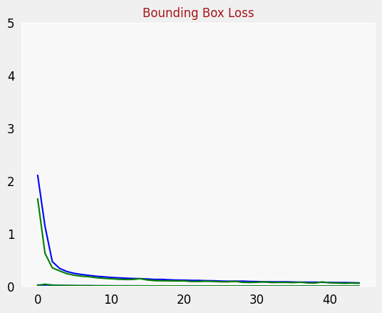
plot_metrics("classification_loss", "Classification Loss")
plot_metrics("bounding_box_loss", "Bounding Box Loss")
Intersection over union
Calculate the I-O-U metric to evaluate the model’s performance.
def intersection_over_union(pred_box, true_box):
    xmin_pred, ymin_pred, xmax_pred, ymax_pred =  np.split(pred_box, 4, axis = 1)
    xmin_true, ymin_true, xmax_true, ymax_true = np.split(true_box, 4, axis = 1)

    smoothing_factor = 1e-10

    xmin_overlap = np.maximum(xmin_pred, xmin_true)
    xmax_overlap = np.minimum(xmax_pred, xmax_true)
    ymin_overlap = np.maximum(ymin_pred, ymin_true)
    ymax_overlap = np.minimum(ymax_pred, ymax_true)

    pred_box_area = (xmax_pred - xmin_pred) * (ymax_pred - ymin_pred)
    true_box_area = (xmax_true - xmin_true) * (ymax_true - ymin_true)

    overlap_area = np.maximum((xmax_overlap - xmin_overlap), 0)  * np.maximum((ymax_overlap - ymin_overlap), 0)
    union_area = (pred_box_area + true_box_area) - overlap_area

    iou = (overlap_area + smoothing_factor) / (union_area + smoothing_factor)

    return iou
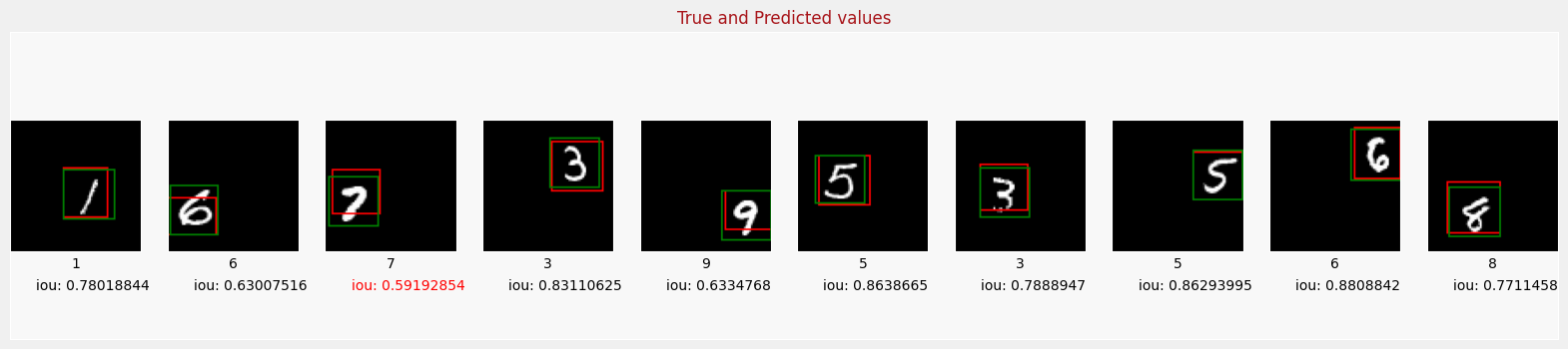
Visualize predictions
The following code will make predictions and visualize both the classification and the predicted bounding boxes.
- The true bounding box labels will be in green, and the model’s predicted bounding boxes are in red.
- The predicted number is shown below the image.
# recognize validation digits
predictions = model.predict(validation_digits, batch_size=64)
predicted_labels = np.argmax(predictions[0], axis=1)

predicted_bboxes = predictions[1]

iou = intersection_over_union(predicted_bboxes, validation_bboxes)

iou_threshold = 0.6

print("Number of predictions where iou > threshold(%s): %s" % (iou_threshold, (iou >= iou_threshold).sum()))
print("Number of predictions where iou < threshold(%s): %s" % (iou_threshold, (iou < iou_threshold).sum()))


display_digits_with_boxes(validation_digits, predicted_labels, validation_labels, predicted_bboxes, validation_bboxes, iou, "True and Predicted values")
157/157 [==============================] - 4s 22ms/step
Number of predictions where iou > threshold(0.6): 9420
Number of predictions where iou < threshold(0.6): 580