Coursera
Predicting Bounding Boxes
Welcome to Course 3, Week 1 Programming Assignment!
In this week’s assignment, you’ll build a model to predict bounding boxes around images.
- You will use transfer learning on any of the pre-trained models available in Keras.
- You’ll be using the Caltech Birds - 2010 dataset.
How to submit your work
Notice that there is not a “submit assignment” button in this notebook.
To check your work and get graded on your work, you’ll train the model, save it and then upload the model to Coursera for grading.
- Initial steps
- 1. Visualization Utilities
- 2. Preprocessing and Loading the Dataset
- 3. Define the Network
- 4. Training the Model
- 5. Validate the Model
- 6. Visualize Predictions
- 7. Upload your model for grading
0. Initial steps
0.1 Set up your Colab
- As you cannot save the changes you make to this colab, you have to make a copy of this notebook in your own drive and run that.
- You can do so by going to
File -> Save a copy in Drive. - Close this colab and open the copy which you have made in your own drive. Then continue to the next step to set up the data location.
Set up the data location
A copy of the dataset that you’ll be using is stored in a publicly viewable Google Drive folder. You’ll want to add a shortcut to it to your own Google Drive.
- Go to this google drive folder named TF3 C3 W1 Data
- Next to the folder name “TF3 C3 W1 Data” (at the top of the page beside “Shared with me”), hover your mouse over the triangle to reveal the drop down menu.
- Use the drop down menu to select
"Add shortcut to Drive"A pop-up menu will open up. - In the pop-up menu, “My Drive” is selected by default. Click the
ADD SHORTCUTbutton. This should add a shortcut to the folderTF3 C3 W1 Datawithin your own Google Drive. - To verify, go to the left-side menu and click on “My Drive”. Scroll through your files to look for the shortcut named
TF3 C3 W1 Data. If the shortcut is namedcaltech_birds2010, then you might have missed a step above and need to repeat the process.
Please make sure the shortcut is created, as you’ll be reading the data for this notebook from this folder.
0.3 Choose the GPU Runtime
- Make sure your runtime is GPU (not CPU or TPU). And if it is an option, make sure you are using Python 3. You can select these settings by going to
Runtime -> Change runtime type -> Select the above mentioned settings and then press SAVE
0.4 Mount your drive
Please run the next code cell and follow these steps to mount your Google Drive so that it can be accessed by this Colab.
- Run the code cell below. A web link will appear below the cell.
- Please click on the web link, which will open a new tab in your browser, which asks you to choose your google account.
- Choose your google account to login.
- The page will display “Google Drive File Stream wants to access your Google Account”. Please click “Allow”.
- The page will now show a code (a line of text). Please copy the code and return to this Colab.
- Paste the code the textbox that is labeled “Enter your authorization code:” and hit
<Enter> - The text will now say “Mounted at /content/drive/”
- Please look at the files explorer of this Colab (left side) and verify that you can navigate to
drive/MyDrive/TF3 C3 W1 Data/caltech_birds2010/0.1.1. If the folder is not there, please redo the steps above and make sure that you’re able to add the shortcut to the hosted dataset.
from google.colab import drive
drive.mount('/content/drive/', force_remount=True)
Mounted at /content/drive/
0.5 Imports
# Install packages for compatibility with the autograder
!pip install tensorflow==2.8.0
!pip install keras==2.8.0
Collecting tensorflow==2.8.0
Downloading tensorflow-2.8.0-cp310-cp310-manylinux2010_x86_64.whl (497.6 MB)
[2K [90m━━━━━━━━━━━━━━━━━━━━━━━━━━━━━━━━━━━━━━━[0m [32m497.6/497.6 MB[0m [31m1.9 MB/s[0m eta [36m0:00:00[0m
[?25hRequirement already satisfied: absl-py>=0.4.0 in /usr/local/lib/python3.10/dist-packages (from tensorflow==2.8.0) (1.4.0)
Requirement already satisfied: astunparse>=1.6.0 in /usr/local/lib/python3.10/dist-packages (from tensorflow==2.8.0) (1.6.3)
Requirement already satisfied: flatbuffers>=1.12 in /usr/local/lib/python3.10/dist-packages (from tensorflow==2.8.0) (23.5.26)
Requirement already satisfied: gast>=0.2.1 in /usr/local/lib/python3.10/dist-packages (from tensorflow==2.8.0) (0.4.0)
Requirement already satisfied: google-pasta>=0.1.1 in /usr/local/lib/python3.10/dist-packages (from tensorflow==2.8.0) (0.2.0)
Requirement already satisfied: h5py>=2.9.0 in /usr/local/lib/python3.10/dist-packages (from tensorflow==2.8.0) (3.9.0)
Collecting keras-preprocessing>=1.1.1 (from tensorflow==2.8.0)
Downloading Keras_Preprocessing-1.1.2-py2.py3-none-any.whl (42 kB)
[2K [90m━━━━━━━━━━━━━━━━━━━━━━━━━━━━━━━━━━━━━━━━[0m [32m42.6/42.6 kB[0m [31m5.2 MB/s[0m eta [36m0:00:00[0m
[?25hRequirement already satisfied: libclang>=9.0.1 in /usr/local/lib/python3.10/dist-packages (from tensorflow==2.8.0) (16.0.6)
Requirement already satisfied: numpy>=1.20 in /usr/local/lib/python3.10/dist-packages (from tensorflow==2.8.0) (1.23.5)
Requirement already satisfied: opt-einsum>=2.3.2 in /usr/local/lib/python3.10/dist-packages (from tensorflow==2.8.0) (3.3.0)
Requirement already satisfied: protobuf>=3.9.2 in /usr/local/lib/python3.10/dist-packages (from tensorflow==2.8.0) (3.20.3)
Requirement already satisfied: setuptools in /usr/local/lib/python3.10/dist-packages (from tensorflow==2.8.0) (67.7.2)
Requirement already satisfied: six>=1.12.0 in /usr/local/lib/python3.10/dist-packages (from tensorflow==2.8.0) (1.16.0)
Requirement already satisfied: termcolor>=1.1.0 in /usr/local/lib/python3.10/dist-packages (from tensorflow==2.8.0) (2.3.0)
Requirement already satisfied: typing-extensions>=3.6.6 in /usr/local/lib/python3.10/dist-packages (from tensorflow==2.8.0) (4.5.0)
Requirement already satisfied: wrapt>=1.11.0 in /usr/local/lib/python3.10/dist-packages (from tensorflow==2.8.0) (1.15.0)
Collecting tensorboard<2.9,>=2.8 (from tensorflow==2.8.0)
Downloading tensorboard-2.8.0-py3-none-any.whl (5.8 MB)
[2K [90m━━━━━━━━━━━━━━━━━━━━━━━━━━━━━━━━━━━━━━━━[0m [32m5.8/5.8 MB[0m [31m75.1 MB/s[0m eta [36m0:00:00[0m
[?25hCollecting tf-estimator-nightly==2.8.0.dev2021122109 (from tensorflow==2.8.0)
Downloading tf_estimator_nightly-2.8.0.dev2021122109-py2.py3-none-any.whl (462 kB)
[2K [90m━━━━━━━━━━━━━━━━━━━━━━━━━━━━━━━━━━━━━━[0m [32m462.5/462.5 kB[0m [31m42.2 MB/s[0m eta [36m0:00:00[0m
[?25hCollecting keras<2.9,>=2.8.0rc0 (from tensorflow==2.8.0)
Downloading keras-2.8.0-py2.py3-none-any.whl (1.4 MB)
[2K [90m━━━━━━━━━━━━━━━━━━━━━━━━━━━━━━━━━━━━━━━━[0m [32m1.4/1.4 MB[0m [31m83.6 MB/s[0m eta [36m0:00:00[0m
[?25hRequirement already satisfied: tensorflow-io-gcs-filesystem>=0.23.1 in /usr/local/lib/python3.10/dist-packages (from tensorflow==2.8.0) (0.34.0)
Requirement already satisfied: grpcio<2.0,>=1.24.3 in /usr/local/lib/python3.10/dist-packages (from tensorflow==2.8.0) (1.58.0)
Requirement already satisfied: wheel<1.0,>=0.23.0 in /usr/local/lib/python3.10/dist-packages (from astunparse>=1.6.0->tensorflow==2.8.0) (0.41.2)
Requirement already satisfied: google-auth<3,>=1.6.3 in /usr/local/lib/python3.10/dist-packages (from tensorboard<2.9,>=2.8->tensorflow==2.8.0) (2.17.3)
Collecting google-auth-oauthlib<0.5,>=0.4.1 (from tensorboard<2.9,>=2.8->tensorflow==2.8.0)
Downloading google_auth_oauthlib-0.4.6-py2.py3-none-any.whl (18 kB)
Requirement already satisfied: markdown>=2.6.8 in /usr/local/lib/python3.10/dist-packages (from tensorboard<2.9,>=2.8->tensorflow==2.8.0) (3.4.4)
Requirement already satisfied: requests<3,>=2.21.0 in /usr/local/lib/python3.10/dist-packages (from tensorboard<2.9,>=2.8->tensorflow==2.8.0) (2.31.0)
Collecting tensorboard-data-server<0.7.0,>=0.6.0 (from tensorboard<2.9,>=2.8->tensorflow==2.8.0)
Downloading tensorboard_data_server-0.6.1-py3-none-manylinux2010_x86_64.whl (4.9 MB)
[2K [90m━━━━━━━━━━━━━━━━━━━━━━━━━━━━━━━━━━━━━━━━[0m [32m4.9/4.9 MB[0m [31m103.0 MB/s[0m eta [36m0:00:00[0m
[?25hCollecting tensorboard-plugin-wit>=1.6.0 (from tensorboard<2.9,>=2.8->tensorflow==2.8.0)
Downloading tensorboard_plugin_wit-1.8.1-py3-none-any.whl (781 kB)
[2K [90m━━━━━━━━━━━━━━━━━━━━━━━━━━━━━━━━━━━━━━[0m [32m781.3/781.3 kB[0m [31m63.2 MB/s[0m eta [36m0:00:00[0m
[?25hRequirement already satisfied: werkzeug>=0.11.15 in /usr/local/lib/python3.10/dist-packages (from tensorboard<2.9,>=2.8->tensorflow==2.8.0) (2.3.7)
Requirement already satisfied: cachetools<6.0,>=2.0.0 in /usr/local/lib/python3.10/dist-packages (from google-auth<3,>=1.6.3->tensorboard<2.9,>=2.8->tensorflow==2.8.0) (5.3.1)
Requirement already satisfied: pyasn1-modules>=0.2.1 in /usr/local/lib/python3.10/dist-packages (from google-auth<3,>=1.6.3->tensorboard<2.9,>=2.8->tensorflow==2.8.0) (0.3.0)
Requirement already satisfied: rsa<5,>=3.1.4 in /usr/local/lib/python3.10/dist-packages (from google-auth<3,>=1.6.3->tensorboard<2.9,>=2.8->tensorflow==2.8.0) (4.9)
Requirement already satisfied: requests-oauthlib>=0.7.0 in /usr/local/lib/python3.10/dist-packages (from google-auth-oauthlib<0.5,>=0.4.1->tensorboard<2.9,>=2.8->tensorflow==2.8.0) (1.3.1)
Requirement already satisfied: charset-normalizer<4,>=2 in /usr/local/lib/python3.10/dist-packages (from requests<3,>=2.21.0->tensorboard<2.9,>=2.8->tensorflow==2.8.0) (3.2.0)
Requirement already satisfied: idna<4,>=2.5 in /usr/local/lib/python3.10/dist-packages (from requests<3,>=2.21.0->tensorboard<2.9,>=2.8->tensorflow==2.8.0) (3.4)
Requirement already satisfied: urllib3<3,>=1.21.1 in /usr/local/lib/python3.10/dist-packages (from requests<3,>=2.21.0->tensorboard<2.9,>=2.8->tensorflow==2.8.0) (2.0.5)
Requirement already satisfied: certifi>=2017.4.17 in /usr/local/lib/python3.10/dist-packages (from requests<3,>=2.21.0->tensorboard<2.9,>=2.8->tensorflow==2.8.0) (2023.7.22)
Requirement already satisfied: MarkupSafe>=2.1.1 in /usr/local/lib/python3.10/dist-packages (from werkzeug>=0.11.15->tensorboard<2.9,>=2.8->tensorflow==2.8.0) (2.1.3)
Requirement already satisfied: pyasn1<0.6.0,>=0.4.6 in /usr/local/lib/python3.10/dist-packages (from pyasn1-modules>=0.2.1->google-auth<3,>=1.6.3->tensorboard<2.9,>=2.8->tensorflow==2.8.0) (0.5.0)
Requirement already satisfied: oauthlib>=3.0.0 in /usr/local/lib/python3.10/dist-packages (from requests-oauthlib>=0.7.0->google-auth-oauthlib<0.5,>=0.4.1->tensorboard<2.9,>=2.8->tensorflow==2.8.0) (3.2.2)
Installing collected packages: tf-estimator-nightly, tensorboard-plugin-wit, keras, tensorboard-data-server, keras-preprocessing, google-auth-oauthlib, tensorboard, tensorflow
Attempting uninstall: keras
Found existing installation: keras 2.13.1
Uninstalling keras-2.13.1:
Successfully uninstalled keras-2.13.1
Attempting uninstall: tensorboard-data-server
Found existing installation: tensorboard-data-server 0.7.1
Uninstalling tensorboard-data-server-0.7.1:
Successfully uninstalled tensorboard-data-server-0.7.1
Attempting uninstall: google-auth-oauthlib
Found existing installation: google-auth-oauthlib 1.0.0
Uninstalling google-auth-oauthlib-1.0.0:
Successfully uninstalled google-auth-oauthlib-1.0.0
Attempting uninstall: tensorboard
Found existing installation: tensorboard 2.13.0
Uninstalling tensorboard-2.13.0:
Successfully uninstalled tensorboard-2.13.0
Attempting uninstall: tensorflow
Found existing installation: tensorflow 2.13.0
Uninstalling tensorflow-2.13.0:
Successfully uninstalled tensorflow-2.13.0
Successfully installed google-auth-oauthlib-0.4.6 keras-2.8.0 keras-preprocessing-1.1.2 tensorboard-2.8.0 tensorboard-data-server-0.6.1 tensorboard-plugin-wit-1.8.1 tensorflow-2.8.0 tf-estimator-nightly-2.8.0.dev2021122109
Requirement already satisfied: keras==2.8.0 in /usr/local/lib/python3.10/dist-packages (2.8.0)
import os, re, time, json
import PIL.Image, PIL.ImageFont, PIL.ImageDraw
import numpy as np
import tensorflow as tf
from matplotlib import pyplot as plt
import tensorflow_datasets as tfds
import cv2
Store the path to the data.
- Remember to follow the steps to
set up the data location(above) so that you’ll have a shortcut to the data in your Google Drive.
data_dir = "/content/drive/My Drive/TF3 C3 W1 Data/"
1. Visualization Utilities
1.1 Bounding Boxes Utilities
We have provided you with some functions which you will use to draw bounding boxes around the birds in the image.
draw_bounding_box_on_image: Draws a single bounding box on an image.draw_bounding_boxes_on_image: Draws multiple bounding boxes on an image.draw_bounding_boxes_on_image_array: Draws multiple bounding boxes on an array of images.
def draw_bounding_box_on_image(image, ymin, xmin, ymax, xmax, color=(255, 0, 0), thickness=5):
    """
    Adds a bounding box to an image.
    Bounding box coordinates can be specified in either absolute (pixel) or
    normalized coordinates by setting the use_normalized_coordinates argument.

    Args:
      image: a PIL.Image object.
      ymin: ymin of bounding box.
      xmin: xmin of bounding box.
      ymax: ymax of bounding box.
      xmax: xmax of bounding box.
      color: color to draw bounding box. Default is red.
      thickness: line thickness. Default value is 4.
    """

    image_width = image.shape[1]
    image_height = image.shape[0]
    cv2.rectangle(image, (int(xmin), int(ymin)), (int(xmax), int(ymax)), color, thickness)


def draw_bounding_boxes_on_image(image, boxes, color=[], thickness=5):
    """
    Draws bounding boxes on image.

    Args:
      image: a PIL.Image object.
      boxes: a 2 dimensional numpy array of [N, 4]: (ymin, xmin, ymax, xmax).
             The coordinates are in normalized format between [0, 1].
      color: color to draw bounding box. Default is red.
      thickness: line thickness. Default value is 4.

    Raises:
      ValueError: if boxes is not a [N, 4] array
    """

    boxes_shape = boxes.shape
    if not boxes_shape:
        return
    if len(boxes_shape) != 2 or boxes_shape[1] != 4:
        raise ValueError('Input must be of size [N, 4]')
    for i in range(boxes_shape[0]):
        draw_bounding_box_on_image(image, boxes[i, 1], boxes[i, 0], boxes[i, 3],
                                 boxes[i, 2], color[i], thickness)


def draw_bounding_boxes_on_image_array(image, boxes, color=[], thickness=5):
    """
    Draws bounding boxes on image (numpy array).

    Args:
      image: a numpy array object.
      boxes: a 2 dimensional numpy array of [N, 4]: (ymin, xmin, ymax, xmax).
             The coordinates are in normalized format between [0, 1].
      color: color to draw bounding box. Default is red.
      thickness: line thickness. Default value is 4.
      display_str_list_list: a list of strings for each bounding box.

    Raises:
      ValueError: if boxes is not a [N, 4] array
    """

    draw_bounding_boxes_on_image(image, boxes, color, thickness)

    return image
1.2 Data and Predictions Utilities
We’ve given you some helper functions and code that are used to visualize the data and the model’s predictions.
display_digits_with_boxes: This displays a row of “digit” images along with the model’s predictions for each image.plot_metrics: This plots a given metric (like loss) as it changes over multiple epochs of training.
# Matplotlib config
plt.rc('image', cmap='gray')
plt.rc('grid', linewidth=0)
plt.rc('xtick', top=False, bottom=False, labelsize='large')
plt.rc('ytick', left=False, right=False, labelsize='large')
plt.rc('axes', facecolor='F8F8F8', titlesize="large", edgecolor='white')
plt.rc('text', color='a8151a')
plt.rc('figure', facecolor='F0F0F0')# Matplotlib fonts
MATPLOTLIB_FONT_DIR = os.path.join(os.path.dirname(plt.__file__), "mpl-data/fonts/ttf")


# utility to display a row of digits with their predictions
def display_digits_with_boxes(images, pred_bboxes, bboxes, iou, title, bboxes_normalized=False):

    n = len(images)

    fig = plt.figure(figsize=(20, 4))
    plt.title(title)
    plt.yticks([])
    plt.xticks([])

    for i in range(n):
      ax = fig.add_subplot(1, 10, i+1)
      bboxes_to_plot = []
      if (len(pred_bboxes) > i):
        bbox = pred_bboxes[i]
        bbox = [bbox[0] * images[i].shape[1], bbox[1] * images[i].shape[0], bbox[2] * images[i].shape[1], bbox[3] * images[i].shape[0]]
        bboxes_to_plot.append(bbox)

      if (len(bboxes) > i):
        bbox = bboxes[i]
        if bboxes_normalized == True:
          bbox = [bbox[0] * images[i].shape[1],bbox[1] * images[i].shape[0], bbox[2] * images[i].shape[1], bbox[3] * images[i].shape[0] ]
        bboxes_to_plot.append(bbox)

      img_to_draw = draw_bounding_boxes_on_image_array(image=images[i], boxes=np.asarray(bboxes_to_plot), color=[(255,0,0), (0, 255, 0)])
      plt.xticks([])
      plt.yticks([])

      plt.imshow(img_to_draw)

      if len(iou) > i :
        color = "black"
        if (iou[i][0] < iou_threshold):
          color = "red"
        ax.text(0.2, -0.3, "iou: %s" %(iou[i][0]), color=color, transform=ax.transAxes)


# utility to display training and validation curves
def plot_metrics(metric_name, title, ylim=5):
    plt.title(title)
    plt.ylim(0,ylim)
    plt.plot(history.history[metric_name],color='blue',label=metric_name)
    plt.plot(history.history['val_' + metric_name],color='green',label='val_' + metric_name)
2. Preprocess and Load the Dataset
2.1 Preprocessing Utilities
We have given you some helper functions to pre-process the image data.
read_image_tfds
- Resizes
imageto (224, 224) - Normalizes
image - Translates and normalizes bounding boxes
def read_image_tfds(image, bbox):
    image = tf.cast(image, tf.float32)
    shape = tf.shape(image)

    factor_x = tf.cast(shape[1], tf.float32)
    factor_y = tf.cast(shape[0], tf.float32)

    image = tf.image.resize(image, (224, 224,))

    image = image/127.5
    image -= 1

    bbox_list = [bbox[0] / factor_x ,
                 bbox[1] / factor_y,
                 bbox[2] / factor_x ,
                 bbox[3] / factor_y]

    return image, bbox_list
read_image_with_shape
This is very similar to read_image_tfds except it also keeps a copy of the original image (before pre-processing) and returns this as well.
- Makes a copy of the original image.
- Resizes
imageto (224, 224) - Normalizes
image - Translates and normalizes bounding boxes
def read_image_with_shape(image, bbox):
    original_image = image

    image, bbox_list = read_image_tfds(image, bbox)

    return original_image, image, bbox_list
read_image_tfds_with_original_bbox
- This function reads
imagefromdata - It also denormalizes the bounding boxes (it undoes the bounding box normalization that is performed by the previous two helper functions.)
def read_image_tfds_with_original_bbox(data):
    image = data["image"]
    bbox = data["bbox"]

    shape = tf.shape(image)
    factor_x = tf.cast(shape[1], tf.float32)
    factor_y = tf.cast(shape[0], tf.float32)

    bbox_list = [bbox[1] * factor_x ,
                 bbox[0] * factor_y,
                 bbox[3] * factor_x,
                 bbox[2] * factor_y]
    return image, bbox_list
dataset_to_numpy_util
This function converts a dataset into numpy arrays of images and boxes.
- This will be used when visualizing the images and their bounding boxes
def dataset_to_numpy_util(dataset, batch_size=0, N=0):

    # eager execution: loop through datasets normally
    take_dataset = dataset.shuffle(1024)

    if batch_size > 0:
        take_dataset = take_dataset.batch(batch_size)

    if N > 0:
        take_dataset = take_dataset.take(N)

    if tf.executing_eagerly():
        ds_images, ds_bboxes = [], []
        for images, bboxes in take_dataset:
            ds_images.append(images.numpy())
            ds_bboxes.append(bboxes.numpy())

    return (np.array(ds_images), np.array(ds_bboxes))
dataset_to_numpy_with_original_bboxes_util
- This function converts a
datasetinto numpy arrays of- original images
- resized and normalized images
- bounding boxes
- This will be used for plotting the original images with true and predicted bounding boxes.
def dataset_to_numpy_with_original_bboxes_util(dataset, batch_size=0, N=0):

    normalized_dataset = dataset.map(read_image_with_shape)
    if batch_size > 0:
        normalized_dataset = normalized_dataset.batch(batch_size)

    if N > 0:
        normalized_dataset = normalized_dataset.take(N)

    if tf.executing_eagerly():
        ds_original_images, ds_images, ds_bboxes = [], [], []

    for original_images, images, bboxes in normalized_dataset:
        ds_images.append(images.numpy())
        ds_bboxes.append(bboxes.numpy())
        ds_original_images.append(original_images.numpy())

    return np.array(ds_original_images), np.array(ds_images), np.array(ds_bboxes)
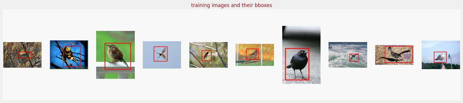
2.2 Visualize the images and their bounding box labels
Now you’ll take a random sample of images from the training and validation sets and visualize them by plotting the corresponding bounding boxes.
Visualize the training images and their bounding box labels
def get_visualization_training_dataset():
    dataset, info = tfds.load("caltech_birds2010", split="train", with_info=True, data_dir=data_dir, download=False)
    print(info)
    visualization_training_dataset = dataset.map(read_image_tfds_with_original_bbox,
                                                 num_parallel_calls=16)
    return visualization_training_dataset


visualization_training_dataset = get_visualization_training_dataset()


(visualization_training_images, visualization_training_bboxes) = dataset_to_numpy_util(visualization_training_dataset, N=10)
display_digits_with_boxes(np.array(visualization_training_images), np.array([]), np.array(visualization_training_bboxes), np.array([]), "training images and their bboxes")
tfds.core.DatasetInfo(
    name='caltech_birds2010',
    full_name='caltech_birds2010/0.1.1',
    description="""
    Caltech-UCSD Birds 200 (CUB-200) is an image dataset with photos
    of 200 bird species (mostly North American). The total number of
    categories of birds is 200 and there are 6033 images in the 2010
    dataset and 11,788 images in the 2011 dataset.
    Annotations include bounding boxes, segmentation labels.
    """,
    homepage='http://www.vision.caltech.edu/visipedia/CUB-200.html',
    data_dir='/content/drive/My Drive/TF3 C3 W1 Data/caltech_birds2010/0.1.1',
    file_format=tfrecord,
    download_size=659.14 MiB,
    dataset_size=659.64 MiB,
    features=FeaturesDict({
        'bbox': BBoxFeature(shape=(4,), dtype=float32),
        'image': Image(shape=(None, None, 3), dtype=uint8),
        'image/filename': Text(shape=(), dtype=string),
        'label': ClassLabel(shape=(), dtype=int64, num_classes=200),
        'label_name': Text(shape=(), dtype=string),
        'segmentation_mask': Image(shape=(None, None, 1), dtype=uint8),
    }),
    supervised_keys=('image', 'label'),
    disable_shuffling=False,
    splits={
        'test': <SplitInfo num_examples=3033, num_shards=4>,
        'train': <SplitInfo num_examples=3000, num_shards=4>,
    },
    citation="""@techreport{WelinderEtal2010,
    Author = {P. Welinder and S. Branson and T. Mita and C. Wah and F. Schroff and S. Belongie and P. Perona},
    Institution = {California Institute of Technology},
    Number = {CNS-TR-2010-001},
    Title = ,
    Year = {2010}
    }""",
)


<ipython-input-10-101de12309d2>:18: VisibleDeprecationWarning: Creating an ndarray from ragged nested sequences (which is a list-or-tuple of lists-or-tuples-or ndarrays with different lengths or shapes) is deprecated. If you meant to do this, you must specify 'dtype=object' when creating the ndarray.
  return (np.array(ds_images), np.array(ds_bboxes))
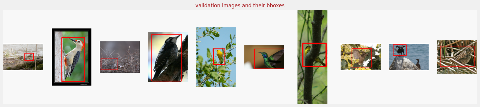
Visualize the validation images and their bounding boxes
def get_visualization_validation_dataset():
    dataset = tfds.load("caltech_birds2010", split="test", data_dir=data_dir, download=False)
    visualization_validation_dataset = dataset.map(read_image_tfds_with_original_bbox, num_parallel_calls=16)
    return visualization_validation_dataset


visualization_validation_dataset = get_visualization_validation_dataset()

(visualization_validation_images, visualization_validation_bboxes) = dataset_to_numpy_util(visualization_validation_dataset, N=10)
display_digits_with_boxes(np.array(visualization_validation_images), np.array([]), np.array(visualization_validation_bboxes), np.array([]), "validation images and their bboxes")
<ipython-input-10-101de12309d2>:18: VisibleDeprecationWarning: Creating an ndarray from ragged nested sequences (which is a list-or-tuple of lists-or-tuples-or ndarrays with different lengths or shapes) is deprecated. If you meant to do this, you must specify 'dtype=object' when creating the ndarray.
  return (np.array(ds_images), np.array(ds_bboxes))
2.3 Load and prepare the datasets for the model
These next two functions read and prepare the datasets that you’ll feed to the model.
- They use
read_image_tfdsto resize, and normalize each image and its bounding box label. - They performs shuffling and batching.
- You’ll use these functions to create
training_datasetandvalidation_dataset, which you will give to the model that you’re about to build.
BATCH_SIZE = 64

def get_training_dataset(dataset):
    dataset = dataset.map(read_image_tfds, num_parallel_calls=16)
    dataset = dataset.shuffle(512, reshuffle_each_iteration=True)
    dataset = dataset.repeat()
    dataset = dataset.batch(BATCH_SIZE)
    dataset = dataset.prefetch(-1)
    return dataset

def get_validation_dataset(dataset):
    dataset = dataset.map(read_image_tfds, num_parallel_calls=16)
    dataset = dataset.batch(BATCH_SIZE)
    dataset = dataset.repeat()
    return dataset

training_dataset = get_training_dataset(visualization_training_dataset)
validation_dataset = get_validation_dataset(visualization_validation_dataset)
3. Define the Network
Bounding box prediction is treated as a “regression” task, in that you want the model to output numerical values.
- You will be performing transfer learning with MobileNet V2. The model architecture is available in TensorFlow Keras.
- You’ll also use pretrained
'imagenet'weights as a starting point for further training. These weights are also readily available - You will choose to retrain all layers of MobileNet V2 along with the final classification layers.
Note: For the following exercises, please use the TensorFlow Keras Functional API (as opposed to the Sequential API).
Exercise 1
Please build a feature extractor using MobileNetV2.
-
First, create an instance of the mobilenet version 2 model
- Please check out the documentation for MobileNetV2
- Set the following parameters:
- input_shape: (height, width, channel): input images have height and width of 224 by 224, and have red, green and blue channels.
- include_top: you do not want to keep the “top” fully connected layer, since you will customize your model for the current task.
- weights: Use the pre-trained ‘imagenet’ weights.
-
Next, make the feature extractor for your specific inputs by passing the
inputsinto your mobilenet model.- For example, if you created a model object called
some_modeland have inputs stored inx, you’d invoke the model and pass in your inputs like this:some_model(x)to get the feature extractor for your given inputsx.
- For example, if you created a model object called
Note: please use mobilenet_v2 and not mobile_net or mobile_net_v3
def feature_extractor(inputs):
    ### YOUR CODE HERE ###

    # Create a mobilenet version 2 model object
    mobilenet_model = tf.keras.applications.mobilenet_v2.MobileNetV2(
        input_shape=(224, 224, 3),
        include_top=False,
        weights="imagenet"
    )


    # pass the inputs into this model object to get a feature extractor for these inputs
    feature_extractor = mobilenet_model(inputs)


    ### END CODE HERE ###

    # return the feature_extractor
    return feature_extractor
Exercise 2
Next, you’ll define the dense layers to be used by your model.
You’ll be using the following layers
- GlobalAveragePooling2D: pools the
features. - Flatten: flattens the pooled layer.
- Dense: Add two dense layers:
- A dense layer with 1024 neurons and a relu activation.
- A dense layer following that with 512 neurons and a relu activation.
Note: Remember, please build the model using the Functional API syntax (as opposed to the Sequential API).
def dense_layers(features):
    ### YOUR CODE HERE ###

    # global average pooling 2d layer
    x = tf.keras.layers.GlobalAveragePooling2D()(features)

    # flatten layer
    x = tf.keras.layers.Flatten()(x)

    # 1024 Dense layer, with relu
    x = tf.keras.layers.Dense(1024, activation="relu")(x)

    # 512 Dense layer, with relu
    x = tf.keras.layers.Dense(512, activation="relu")(x)

    ### END CODE HERE ###

    return x
Exercise 3
Now you’ll define a layer that outputs the bounding box predictions.
- You’ll use a Dense layer.
- Remember that you have 4 units in the output layer, corresponding to (xmin, ymin, xmax, ymax).
- The prediction layer follows the previous dense layer, which is passed into this function as the variable
x. - For grading purposes, please set the
nameparameter of this Dense layer to be `bounding_box’
def bounding_box_regression(x):
    ### YOUR CODE HERE ###

    # Dense layer named `bounding_box`
    bounding_box_regression_output = tf.keras.layers.Dense(4, name="bounding_box")(x)

    ### END CODE HERE ###


    return bounding_box_regression_output
Exercise 4
Now, you’ll use those functions that you have just defined above to construct the model.
- feature_extractor(inputs)
- dense_layers(features)
- bounding_box_regression(x)
Then you’ll define the model object using Model. Set the two parameters:
- inputs
- outputs
def final_model(inputs):
    ### YOUR CODE HERE ###

    # features
    feature_cnn = feature_extractor(inputs)

    # dense layers
    last_dense_layer = dense_layers(feature_cnn)

    # bounding box
    bounding_box_output = bounding_box_regression(last_dense_layer)

    # define the TensorFlow Keras model using the inputs and outputs to your model
    model = tf.keras.Model(inputs=inputs, outputs=bounding_box_output)

    ### END CODE HERE ###


    return model
Exercise 5
Define the input layer, define the model, and then compile the model.
- inputs: define an Input layer
- Set the
shapeparameter. Check your definition offeature_extractorto see the expected dimensions of the input image.
- Set the
- model: use the
final_modelfunction that you just defined to create the model. - compile the model: Check the Model documentation for how to compile the model.
- Set the
optimizerparameter to Stochastic Gradient Descent using SGD- When using SGD, set the
momentumto 0.9 and keep the default learning rate. (Note: To avoid grading issues, please usetf.keras.optimizers.SGDinstead oftf.keras.optimizers.experimental.SGD. We will remove this note once the grader has been updated to recognize theexperimentalmodule.).
- When using SGD, set the
- Set the loss function of SGD to mean squared error (see the SGD documentation for an example of how to choose mean squared error loss).
- Set the
def define_and_compile_model():

    ### YOUR CODE HERE ###

    # define the input layer
    inputs = tf.keras.layers.Input(shape=(224, 224, 3))

    # create the model
    model = final_model(inputs)

    # compile your model
    model.compile(
        optimizer=tf.keras.optimizers.SGD(momentum=.9),
        loss="mse"
    )

    ### END CODE HERE ###


    return model
Run the cell below to define your model and print the model summary.
# define your model
model = define_and_compile_model()
# print model layers
model.summary()
Downloading data from https://storage.googleapis.com/tensorflow/keras-applications/mobilenet_v2/mobilenet_v2_weights_tf_dim_ordering_tf_kernels_1.0_224_no_top.h5
9412608/9406464 [==============================] - 0s 0us/step
9420800/9406464 [==============================] - 0s 0us/step
Model: "model"
_________________________________________________________________
 Layer (type)                Output Shape              Param #
=================================================================
 input_1 (InputLayer)        [(None, 224, 224, 3)]     0

 mobilenetv2_1.00_224 (Funct  (None, 7, 7, 1280)       2257984
 ional)

 global_average_pooling2d (G  (None, 1280)             0
 lobalAveragePooling2D)

 flatten (Flatten)           (None, 1280)              0

 dense (Dense)               (None, 1024)              1311744

 dense_1 (Dense)             (None, 512)               524800

 bounding_box (Dense)        (None, 4)                 2052

=================================================================
Total params: 4,096,580
Trainable params: 4,062,468
Non-trainable params: 34,112
_________________________________________________________________
Your expected model summary:

Train the Model
4.1 Prepare to Train the Model
You’ll fit the model here, but first you’ll set some of the parameters that go into fitting the model.
-
EPOCHS: You’ll train the model for 50 epochs
-
BATCH_SIZE: Set the
BATCH_SIZEto an appropriate value. You can look at the ungraded labs from this week for some examples. -
length_of_training_dataset: this is the number of training examples. You can find this value by getting the length of
visualization_training_dataset.- Note: You won’t be able to get the length of the object
training_dataset. (You’ll get an error message).
- Note: You won’t be able to get the length of the object
-
length_of_validation_dataset: this is the number of validation examples. You can find this value by getting the length of
visualization_validation_dataset.- Note: You won’t be able to get the length of the object
validation_dataset.
- Note: You won’t be able to get the length of the object
-
steps_per_epoch: This is the number of steps it will take to process all of the training data.
- If the number of training examples is not evenly divisible by the batch size, there will be one last batch that is not the full batch size.
- Try to calculate the number steps it would take to train all the full batches plus one more batch containing the remaining training examples. There are a couples ways you can calculate this.
- You can use regular division
/and importmathto usemath.ceil()Python math module docs - Alternatively, you can use
//for integer division,%to check for a remainder after integer division, and anifstatement.
- You can use regular division
-
validation_steps: This is the number of steps it will take to process all of the validation data. You can use similar calculations that you did for the step_per_epoch, but for the validation dataset.
Exercise 6
# You'll train 50 epochs
EPOCHS = 50

### START CODE HERE ###

# Choose a batch size
BATCH_SIZE = 64

# Get the length of the training set
length_of_training_dataset = len(visualization_training_dataset)

# Get the length of the validation set
length_of_validation_dataset = len(visualization_validation_dataset)

# Get the steps per epoch (may be a few lines of code)
steps_per_epoch = length_of_training_dataset // BATCH_SIZE
if length_of_training_dataset % BATCH_SIZE > 0:
    steps_per_epoch += 1

# get the validation steps (per epoch) (may be a few lines of code)
validation_steps = length_of_validation_dataset//BATCH_SIZE
if length_of_validation_dataset % BATCH_SIZE > 0:
    validation_steps += 1

### END CODE HERE
4.2 Fit the model to the data
Check out the parameters that you can set to fit the Model. Please set the following parameters.
- x: this can be a tuple of both the features and labels, as is the case here when using a tf.Data dataset.
- Please use the variable returned from
get_training_dataset(). - Note, don’t set the
yparameter when thexis already set to both the features and labels.
- Please use the variable returned from
- steps_per_epoch: the number of steps to train in order to train on all examples in the training dataset.
- validation_data: this is a tuple of both the features and labels of the validation set.
- Please use the variable returned from
get_validation_dataset()
- Please use the variable returned from
- validation_steps: teh number of steps to go through the validation set, batch by batch.
- epochs: the number of epochs.
If all goes well your model’s training will start.
Exercise 7
### YOUR CODE HERE ####

# Fit the model, setting the parameters noted in the instructions above.
history = model.fit(x=training_dataset,
                    steps_per_epoch=steps_per_epoch,
                    validation_data=validation_dataset,
                    validation_steps=validation_steps,
                    epochs=EPOCHS)

### END CODE HERE ###
Epoch 1/50
47/47 [==============================] - 56s 793ms/step - loss: 0.0767 - val_loss: 0.2079
Epoch 2/50
47/47 [==============================] - 45s 961ms/step - loss: 0.0195 - val_loss: 0.1999
Epoch 3/50
47/47 [==============================] - 38s 813ms/step - loss: 0.0127 - val_loss: 0.1524
Epoch 4/50
47/47 [==============================] - 39s 839ms/step - loss: 0.0095 - val_loss: 0.1425
Epoch 5/50
47/47 [==============================] - 38s 818ms/step - loss: 0.0079 - val_loss: 0.1237
Epoch 6/50
47/47 [==============================] - 36s 770ms/step - loss: 0.0067 - val_loss: 0.1071
Epoch 7/50
47/47 [==============================] - 36s 766ms/step - loss: 0.0059 - val_loss: 0.0957
Epoch 8/50
47/47 [==============================] - 36s 764ms/step - loss: 0.0055 - val_loss: 0.0853
Epoch 9/50
47/47 [==============================] - 39s 842ms/step - loss: 0.0049 - val_loss: 0.0735
Epoch 10/50
47/47 [==============================] - 34s 735ms/step - loss: 0.0046 - val_loss: 0.0661
Epoch 11/50
47/47 [==============================] - 39s 832ms/step - loss: 0.0042 - val_loss: 0.0562
Epoch 12/50
47/47 [==============================] - 35s 760ms/step - loss: 0.0040 - val_loss: 0.0512
Epoch 13/50
47/47 [==============================] - 39s 837ms/step - loss: 0.0037 - val_loss: 0.0484
Epoch 14/50
47/47 [==============================] - 36s 762ms/step - loss: 0.0036 - val_loss: 0.0460
Epoch 15/50
47/47 [==============================] - 36s 771ms/step - loss: 0.0034 - val_loss: 0.0460
Epoch 16/50
47/47 [==============================] - 36s 771ms/step - loss: 0.0031 - val_loss: 0.0373
Epoch 17/50
47/47 [==============================] - 35s 759ms/step - loss: 0.0031 - val_loss: 0.0386
Epoch 18/50
47/47 [==============================] - 43s 921ms/step - loss: 0.0031 - val_loss: 0.0344
Epoch 19/50
47/47 [==============================] - 35s 760ms/step - loss: 0.0030 - val_loss: 0.0337
Epoch 20/50
47/47 [==============================] - 35s 757ms/step - loss: 0.0030 - val_loss: 0.0345
Epoch 21/50
47/47 [==============================] - 35s 756ms/step - loss: 0.0029 - val_loss: 0.0302
Epoch 22/50
47/47 [==============================] - 36s 767ms/step - loss: 0.0028 - val_loss: 0.0299
Epoch 23/50
47/47 [==============================] - 35s 752ms/step - loss: 0.0026 - val_loss: 0.0293
Epoch 24/50
47/47 [==============================] - 38s 817ms/step - loss: 0.0027 - val_loss: 0.0273
Epoch 25/50
47/47 [==============================] - 35s 750ms/step - loss: 0.0027 - val_loss: 0.0288
Epoch 26/50
47/47 [==============================] - 35s 753ms/step - loss: 0.0026 - val_loss: 0.0269
Epoch 27/50
47/47 [==============================] - 35s 760ms/step - loss: 0.0026 - val_loss: 0.0242
Epoch 28/50
47/47 [==============================] - 39s 844ms/step - loss: 0.0024 - val_loss: 0.0246
Epoch 29/50
47/47 [==============================] - 34s 737ms/step - loss: 0.0024 - val_loss: 0.0238
Epoch 30/50
47/47 [==============================] - 34s 736ms/step - loss: 0.0024 - val_loss: 0.0234
Epoch 31/50
47/47 [==============================] - 36s 775ms/step - loss: 0.0024 - val_loss: 0.0226
Epoch 32/50
47/47 [==============================] - 35s 748ms/step - loss: 0.0022 - val_loss: 0.0229
Epoch 33/50
47/47 [==============================] - 35s 755ms/step - loss: 0.0024 - val_loss: 0.0216
Epoch 34/50
47/47 [==============================] - 39s 839ms/step - loss: 0.0023 - val_loss: 0.0208
Epoch 35/50
47/47 [==============================] - 35s 747ms/step - loss: 0.0021 - val_loss: 0.0206
Epoch 36/50
47/47 [==============================] - 34s 735ms/step - loss: 0.0022 - val_loss: 0.0206
Epoch 37/50
47/47 [==============================] - 34s 737ms/step - loss: 0.0021 - val_loss: 0.0206
Epoch 38/50
47/47 [==============================] - 37s 796ms/step - loss: 0.0021 - val_loss: 0.0203
Epoch 39/50
47/47 [==============================] - 34s 729ms/step - loss: 0.0021 - val_loss: 0.0196
Epoch 40/50
47/47 [==============================] - 35s 754ms/step - loss: 0.0020 - val_loss: 0.0196
Epoch 41/50
47/47 [==============================] - 35s 746ms/step - loss: 0.0021 - val_loss: 0.0190
Epoch 42/50
47/47 [==============================] - 35s 755ms/step - loss: 0.0019 - val_loss: 0.0190
Epoch 43/50
47/47 [==============================] - 39s 848ms/step - loss: 0.0020 - val_loss: 0.0183
Epoch 44/50
47/47 [==============================] - 35s 745ms/step - loss: 0.0019 - val_loss: 0.0191
Epoch 45/50
47/47 [==============================] - 37s 802ms/step - loss: 0.0020 - val_loss: 0.0186
Epoch 46/50
47/47 [==============================] - 36s 764ms/step - loss: 0.0020 - val_loss: 0.0187
Epoch 47/50
47/47 [==============================] - 35s 751ms/step - loss: 0.0019 - val_loss: 0.0184
Epoch 48/50
47/47 [==============================] - 39s 842ms/step - loss: 0.0019 - val_loss: 0.0178
Epoch 49/50
47/47 [==============================] - 35s 750ms/step - loss: 0.0018 - val_loss: 0.0178
Epoch 50/50
47/47 [==============================] - 35s 755ms/step - loss: 0.0018 - val_loss: 0.0180
5. Validate the Model
5.1 Loss
You can now evaluate your trained model’s performance by checking its loss value on the validation set.
loss = model.evaluate(validation_dataset, steps=validation_steps)
print("Loss: ", loss)
48/48 [==============================] - 14s 289ms/step - loss: 0.0180
Loss:  0.018038643524050713
5.2 Save your Model for Grading
When you have trained your model and are satisfied with your validation loss, please you save your model so that you can upload it to the Coursera classroom for grading.
# Please save your model
model.save("birds.h5")
# And download it using this shortcut or from the "Files" panel to the left
from google.colab import files

files.download("birds.h5")
<IPython.core.display.Javascript object>


<IPython.core.display.Javascript object>
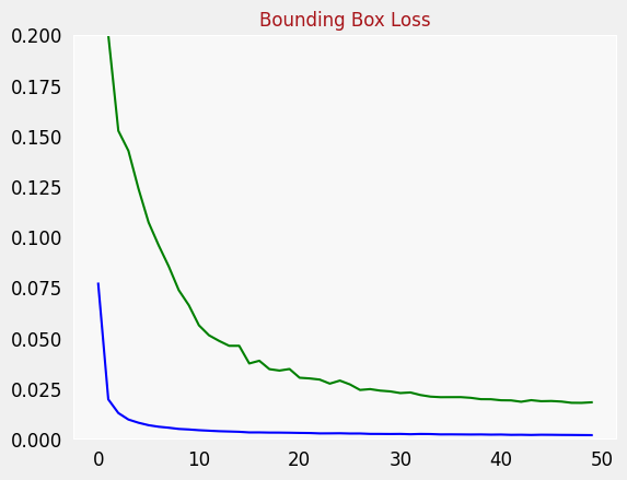
5.3 Plot Loss Function
You can also plot the loss metrics.
plot_metrics("loss", "Bounding Box Loss", ylim=0.2)
5.4 Evaluate performance using IoU
You can see how well your model predicts bounding boxes on the validation set by calculating the Intersection-over-union (IoU) score for each image.
- You’ll find the IoU calculation implemented for you.
- Predict on the validation set of images.
- Apply the
intersection_over_unionon these predicted bounding boxes.
def intersection_over_union(pred_box, true_box):

    xmin_pred, ymin_pred, xmax_pred, ymax_pred =  np.split(pred_box, 4, axis = 1)
    xmin_true, ymin_true, xmax_true, ymax_true = np.split(true_box, 4, axis = 1)

    #Calculate coordinates of overlap area between boxes
    xmin_overlap = np.maximum(xmin_pred, xmin_true)
    xmax_overlap = np.minimum(xmax_pred, xmax_true)
    ymin_overlap = np.maximum(ymin_pred, ymin_true)
    ymax_overlap = np.minimum(ymax_pred, ymax_true)

    #Calculates area of true and predicted boxes
    pred_box_area = (xmax_pred - xmin_pred) * (ymax_pred - ymin_pred)
    true_box_area = (xmax_true - xmin_true) * (ymax_true - ymin_true)

    #Calculates overlap area and union area.
    overlap_area = np.maximum((xmax_overlap - xmin_overlap),0)  * np.maximum((ymax_overlap - ymin_overlap), 0)
    union_area = (pred_box_area + true_box_area) - overlap_area

    # Defines a smoothing factor to prevent division by 0
    smoothing_factor = 1e-10

    #Updates iou score
    iou = (overlap_area + smoothing_factor) / (union_area + smoothing_factor)

    return iou

#Makes predictions
original_images, normalized_images, normalized_bboxes = dataset_to_numpy_with_original_bboxes_util(visualization_validation_dataset, N=500)
predicted_bboxes = model.predict(normalized_images, batch_size=32)


#Calculates IOU and reports true positives and false positives based on IOU threshold
iou = intersection_over_union(predicted_bboxes, normalized_bboxes)
iou_threshold = 0.5

print("Number of predictions where iou > threshold(%s): %s" % (iou_threshold, (iou >= iou_threshold).sum()))
print("Number of predictions where iou < threshold(%s): %s" % (iou_threshold, (iou < iou_threshold).sum()))
<ipython-input-11-0f92292fe070>:18: VisibleDeprecationWarning: Creating an ndarray from ragged nested sequences (which is a list-or-tuple of lists-or-tuples-or ndarrays with different lengths or shapes) is deprecated. If you meant to do this, you must specify 'dtype=object' when creating the ndarray.
  return np.array(ds_original_images), np.array(ds_images), np.array(ds_bboxes)


Number of predictions where iou > threshold(0.5): 240
Number of predictions where iou < threshold(0.5): 260
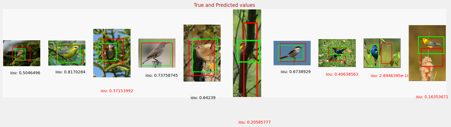
6. Visualize Predictions
Lastly, you’ll plot the predicted and ground truth bounding boxes for a random set of images and visually see how well you did!
n = 10
indexes = np.random.choice(len(predicted_bboxes), size=n)

iou_to_draw = iou[indexes]
norm_to_draw = original_images[indexes]
display_digits_with_boxes(original_images[indexes], predicted_bboxes[indexes], normalized_bboxes[indexes], iou[indexes], "True and Predicted values", bboxes_normalized=True)
7 Upload your model for grading
Please return to the Coursera classroom and find the section that allows you to upload your ‘birds.h5’ model for grading. Good luck!