Coursera
Week 3 Assignment: Image Segmentation of Handwritten Digits
In this week’s assignment, you will build a model that predicts the segmentation masks (pixel-wise label map) of handwritten digits. This model will be trained on the M2NIST dataset, a multi digit MNIST. If you’ve done the ungraded lab on the CamVid dataset, then many of the steps here will look familiar.
You will build a Convolutional Neural Network (CNN) from scratch for the downsampling path and use a Fully Convolutional Network, FCN-8, to upsample and produce the pixel-wise label map. The model will be evaluated using the intersection over union (IOU) and Dice Score. Finally, you will download the model and upload it to the grader in Coursera to get your score for the assignment.
Exercises
We’ve given you some boilerplate code to work with and these are the 5 exercises you need to fill out before you can successfully get the segmentation masks.
- Exercise 1 - Define the Basic Convolution Block
- Exercise 2 - Define the Downsampling Path
- Exercise 3 - Define the FCN-8 decoder
- Exercise 4 - Compile the Model
- Exercise 5 - Model Training
Imports
As usual, let’s start by importing the packages you will use in this lab.
# Install packages for compatibility with the autograder

# NOTE: You can safely ignore errors about version incompatibility of
# Colab-bundled packages (e.g. xarray, pydantic, etc.)

!pip install tensorflow==2.8.0 --quiet
!pip install keras==2.8.0 --quiet
[2K [90m━━━━━━━━━━━━━━━━━━━━━━━━━━━━━━━━━━━━━━━[0m [32m497.6/497.6 MB[0m [31m2.2 MB/s[0m eta [36m0:00:00[0m
[2K [90m━━━━━━━━━━━━━━━━━━━━━━━━━━━━━━━━━━━━━━━━[0m [32m42.6/42.6 kB[0m [31m4.0 MB/s[0m eta [36m0:00:00[0m
[2K [90m━━━━━━━━━━━━━━━━━━━━━━━━━━━━━━━━━━━━━━━━[0m [32m5.8/5.8 MB[0m [31m54.1 MB/s[0m eta [36m0:00:00[0m
[2K [90m━━━━━━━━━━━━━━━━━━━━━━━━━━━━━━━━━━━━━━[0m [32m462.5/462.5 kB[0m [31m14.6 MB/s[0m eta [36m0:00:00[0m
[2K [90m━━━━━━━━━━━━━━━━━━━━━━━━━━━━━━━━━━━━━━━━[0m [32m1.4/1.4 MB[0m [31m51.4 MB/s[0m eta [36m0:00:00[0m
[2K [90m━━━━━━━━━━━━━━━━━━━━━━━━━━━━━━━━━━━━━━━━[0m [32m4.9/4.9 MB[0m [31m48.9 MB/s[0m eta [36m0:00:00[0m
[2K [90m━━━━━━━━━━━━━━━━━━━━━━━━━━━━━━━━━━━━━━[0m [32m781.3/781.3 kB[0m [31m52.7 MB/s[0m eta [36m0:00:00[0m
[?25h
try:
  # %tensorflow_version only exists in Colab.
  %tensorflow_version 2.x
except Exception:
  pass

import os
import zipfile

import PIL.Image, PIL.ImageFont, PIL.ImageDraw
import numpy as np
from matplotlib import pyplot as plt

import tensorflow as tf
import tensorflow_datasets as tfds
from sklearn.model_selection import train_test_split

print("Tensorflow version " + tf.__version__)
Colab only includes TensorFlow 2.x; %tensorflow_version has no effect.
Tensorflow version 2.8.0
Download the dataset
M2NIST is a multi digit MNIST. Each image has up to 3 digits from MNIST digits and the corresponding labels file has the segmentation masks.
The dataset is available on Kaggle and you can find it here
To make it easier for you, we’re hosting it on Google Cloud so you can download without Kaggle credentials.
# download zipped dataset
!wget --no-check-certificate \
    https://storage.googleapis.com/tensorflow-1-public/tensorflow-3-temp/m2nist.zip \
    -O /tmp/m2nist.zip

# find and extract to a local folder ('/tmp/training')
local_zip = '/tmp/m2nist.zip'
zip_ref = zipfile.ZipFile(local_zip, 'r')
zip_ref.extractall('/tmp/training')
zip_ref.close()
--2023-10-04 16:39:38--  https://storage.googleapis.com/tensorflow-1-public/tensorflow-3-temp/m2nist.zip
Resolving storage.googleapis.com (storage.googleapis.com)... 108.177.127.207, 142.251.31.207, 74.125.128.207, ...
Connecting to storage.googleapis.com (storage.googleapis.com)|108.177.127.207|:443... connected.
HTTP request sent, awaiting response... 200 OK
Length: 17378168 (17M) [application/zip]
Saving to: ‘/tmp/m2nist.zip’

/tmp/m2nist.zip     100%[===================>]  16.57M  17.7MB/s    in 0.9s

2023-10-04 16:39:40 (17.7 MB/s) - ‘/tmp/m2nist.zip’ saved [17378168/17378168]
Load and Preprocess the Dataset
This dataset can be easily preprocessed since it is available as Numpy Array Files (.npy)
-
combined.npy has the image files containing the multiple MNIST digits. Each image is of size 64 x 84 (height x width, in pixels).
-
segmented.npy has the corresponding segmentation masks. Each segmentation mask is also of size 64 x 84.
This dataset has 5000 samples and you can make appropriate training, validation, and test splits as required for the problem.
With that, let’s define a few utility functions for loading and preprocessing the dataset.
BATCH_SIZE = 32

def read_image_and_annotation(image, annotation):
  '''
  Casts the image and annotation to their expected data type and
  normalizes the input image so that each pixel is in the range [-1, 1]

  Args:
    image (numpy array) -- input image
    annotation (numpy array) -- ground truth label map

  Returns:
    preprocessed image-annotation pair
  '''

  image = tf.cast(image, dtype=tf.float32)
  image = tf.reshape(image, (image.shape[0], image.shape[1], 1,))
  annotation = tf.cast(annotation, dtype=tf.int32)
  image = image / 127.5
  image -= 1

  return image, annotation


def get_training_dataset(images, annos):
  '''
  Prepares shuffled batches of the training set.

  Args:
    images (list of strings) -- paths to each image file in the train set
    annos (list of strings) -- paths to each label map in the train set

  Returns:
    tf Dataset containing the preprocessed train set
  '''
  training_dataset = tf.data.Dataset.from_tensor_slices((images, annos))
  training_dataset = training_dataset.map(read_image_and_annotation)

  training_dataset = training_dataset.shuffle(512, reshuffle_each_iteration=True)
  training_dataset = training_dataset.batch(BATCH_SIZE)
  training_dataset = training_dataset.repeat()
  training_dataset = training_dataset.prefetch(-1)

  return training_dataset


def get_validation_dataset(images, annos):
  '''
  Prepares batches of the validation set.

  Args:
    images (list of strings) -- paths to each image file in the val set
    annos (list of strings) -- paths to each label map in the val set

  Returns:
    tf Dataset containing the preprocessed validation set
  '''
  validation_dataset = tf.data.Dataset.from_tensor_slices((images, annos))
  validation_dataset = validation_dataset.map(read_image_and_annotation)
  validation_dataset = validation_dataset.batch(BATCH_SIZE)
  validation_dataset = validation_dataset.repeat()

  return validation_dataset


def get_test_dataset(images, annos):
  '''
  Prepares batches of the test set.

  Args:
    images (list of strings) -- paths to each image file in the test set
    annos (list of strings) -- paths to each label map in the test set

  Returns:
    tf Dataset containing the preprocessed validation set
  '''
  test_dataset = tf.data.Dataset.from_tensor_slices((images, annos))
  test_dataset = test_dataset.map(read_image_and_annotation)
  test_dataset = test_dataset.batch(BATCH_SIZE, drop_remainder=True)

  return test_dataset


def load_images_and_segments():
  '''
  Loads the images and segments as numpy arrays from npy files
  and makes splits for training, validation and test datasets.

  Returns:
    3 tuples containing the train, val, and test splits
  '''

  #Loads images and segmentation masks.
  images = np.load('/tmp/training/combined.npy')
  segments = np.load('/tmp/training/segmented.npy')

  #Makes training, validation, test splits from loaded images and segmentation masks.
  train_images, val_images, train_annos, val_annos = train_test_split(images, segments, test_size=0.2, shuffle=True)
  val_images, test_images, val_annos, test_annos = train_test_split(val_images, val_annos, test_size=0.2, shuffle=True)

  return (train_images, train_annos), (val_images, val_annos), (test_images, test_annos)
You can now load the preprocessed dataset and define the training, validation, and test sets.
# Load Dataset
train_slices, val_slices, test_slices = load_images_and_segments()

# Create training, validation, test datasets.
training_dataset = get_training_dataset(train_slices[0], train_slices[1])
validation_dataset = get_validation_dataset(val_slices[0], val_slices[1])
test_dataset = get_test_dataset(test_slices[0], test_slices[1])
Let’s Take a Look at the Dataset
You may want to visually inspect the dataset before and after training. Like above, we’ve included utility functions to help show a few images as well as their annotations (i.e. labels).
# Visualization Utilities

# there are 11 classes in the dataset: one class for each digit (0 to 9) plus the background class
n_classes = 11

# assign a random color for each class
colors = [tuple(np.random.randint(256, size=3) / 255.0) for i in range(n_classes)]

def fuse_with_pil(images):
  '''
  Creates a blank image and pastes input images

  Args:
    images (list of numpy arrays) - numpy array representations of the images to paste

  Returns:
    PIL Image object containing the images
  '''

  widths = (image.shape[1] for image in images)
  heights = (image.shape[0] for image in images)
  total_width = sum(widths)
  max_height = max(heights)

  new_im = PIL.Image.new('RGB', (total_width, max_height))

  x_offset = 0
  for im in images:
    pil_image = PIL.Image.fromarray(np.uint8(im))
    new_im.paste(pil_image, (x_offset,0))
    x_offset += im.shape[1]

  return new_im


def give_color_to_annotation(annotation):
  '''
  Converts a 2-D annotation to a numpy array with shape (height, width, 3) where
  the third axis represents the color channel. The label values are multiplied by
  255 and placed in this axis to give color to the annotation

  Args:
    annotation (numpy array) - label map array

  Returns:
    the annotation array with an additional color channel/axis
  '''
  seg_img = np.zeros( (annotation.shape[0],annotation.shape[1], 3) ).astype('float')

  for c in range(n_classes):
    segc = (annotation == c)
    seg_img[:,:,0] += segc*( colors[c][0] * 255.0)
    seg_img[:,:,1] += segc*( colors[c][1] * 255.0)
    seg_img[:,:,2] += segc*( colors[c][2] * 255.0)

  return seg_img


def show_annotation_and_prediction(image, annotation, prediction, iou_list, dice_score_list):
  '''
  Displays the images with the ground truth and predicted label maps. Also overlays the metrics.

  Args:
    image (numpy array) -- the input image
    annotation (numpy array) -- the ground truth label map
    prediction (numpy array) -- the predicted label map
    iou_list (list of floats) -- the IOU values for each class
    dice_score_list (list of floats) -- the Dice Score for each class
  '''

  new_ann = np.argmax(annotation, axis=2)
  true_img = give_color_to_annotation(new_ann)
  pred_img = give_color_to_annotation(prediction)

  image = image + 1
  image = image * 127.5
  image = np.reshape(image, (image.shape[0], image.shape[1],))
  image = np.uint8(image)
  images = [image, np.uint8(pred_img), np.uint8(true_img)]

  metrics_by_id = [(idx, iou, dice_score) for idx, (iou, dice_score) in enumerate(zip(iou_list, dice_score_list)) if iou > 0.0 and idx < 10]
  metrics_by_id.sort(key=lambda tup: tup[1], reverse=True)  # sorts in place

  display_string_list = ["{}: IOU: {} Dice Score: {}".format(idx, iou, dice_score) for idx, iou, dice_score in metrics_by_id]
  display_string = "\n".join(display_string_list)

  plt.figure(figsize=(15, 4))

  for idx, im in enumerate(images):
    plt.subplot(1, 3, idx+1)
    if idx == 1:
      plt.xlabel(display_string)
    plt.xticks([])
    plt.yticks([])
    plt.imshow(im)


def show_annotation_and_image(image, annotation):
  '''
  Displays the image and its annotation side by side

  Args:
    image (numpy array) -- the input image
    annotation (numpy array) -- the label map
  '''
  new_ann = np.argmax(annotation, axis=2)
  seg_img = give_color_to_annotation(new_ann)

  image = image + 1
  image = image * 127.5
  image = np.reshape(image, (image.shape[0], image.shape[1],))

  image = np.uint8(image)
  images = [image, seg_img]

  images = [image, seg_img]
  fused_img = fuse_with_pil(images)
  plt.imshow(fused_img)


def list_show_annotation(dataset, num_images):
  '''
  Displays images and its annotations side by side

  Args:
    dataset (tf Dataset) -- batch of images and annotations
    num_images (int) -- number of images to display
  '''
  ds = dataset.unbatch()

  plt.figure(figsize=(20, 15))
  plt.title("Images And Annotations")
  plt.subplots_adjust(bottom=0.1, top=0.9, hspace=0.05)

  for idx, (image, annotation) in enumerate(ds.take(num_images)):
    plt.subplot(5, 5, idx + 1)
    plt.yticks([])
    plt.xticks([])
    show_annotation_and_image(image.numpy(), annotation.numpy())
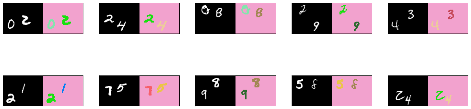
You can view a subset of the images from the dataset with the list_show_annotation() function defined above. Run the cells below to see the image on the left and its pixel-wise ground truth label map on the right.
# get 10 images from the training set
list_show_annotation(training_dataset, 10)
<ipython-input-6-dc81ed44ba48>:136: MatplotlibDeprecationWarning: Auto-removal of overlapping axes is deprecated since 3.6 and will be removed two minor releases later; explicitly call ax.remove() as needed.
  plt.subplot(5, 5, idx + 1)
# get 10 images from the validation set
list_show_annotation(validation_dataset, 10)
<ipython-input-6-dc81ed44ba48>:136: MatplotlibDeprecationWarning: Auto-removal of overlapping axes is deprecated since 3.6 and will be removed two minor releases later; explicitly call ax.remove() as needed.
  plt.subplot(5, 5, idx + 1)
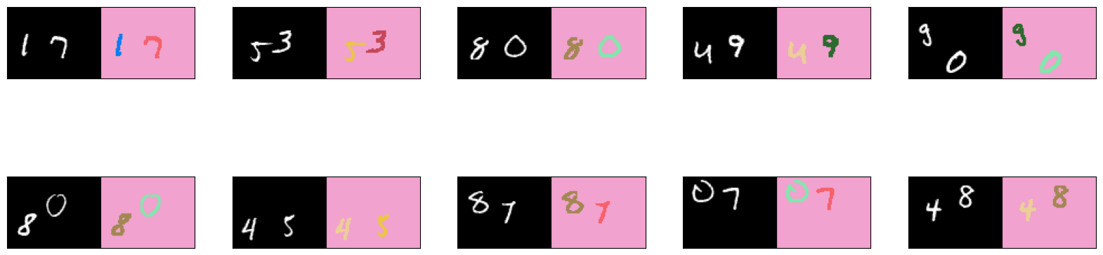
You see from the images above the colors assigned to each class (i.e 0 to 9 plus the background). If you don’t like these colors, feel free to rerun the cell where colors is defined to get another set of random colors. Alternatively, you can assign the RGB values for each class instead of relying on random values.
Define the Model
As discussed in the lectures, the image segmentation model will have two paths:
-
Downsampling Path - This part of the network extracts the features in the image. This is done through a series of convolution and pooling layers. The final output is a reduced image (because of the pooling layers) with the extracted features. You will build a custom CNN from scratch for this path.
-
Upsampling Path - This takes the output of the downsampling path and generates the predictions while also converting the image back to its original size. You will use an FCN-8 decoder for this path.
Define the Basic Convolution Block
Exercise 1
Please complete the function below to build the basic convolution block for our CNN. This will have two Conv2D layers each followed by a LeakyReLU, then max pooled and batch-normalized. Use the functional syntax to stack these layers.
$$Input -> Conv2D -> LeakyReLU -> Conv2D -> LeakyReLU -> MaxPooling2D -> BatchNormalization$$
When defining the Conv2D layers, note that our data inputs will have the ‘channels’ dimension last. You may want to check the data_format argument in the docs regarding this. Take note of the padding argument too like you did in the ungraded labs.
Lastly, to use the LeakyReLU activation, you do not need to nest it inside an Activation layer (e.g. x = tf.keras.layers.Activation(tf.keras.layers.LeakyReLU()(x)). You can simply stack the layer directly instead (e.g. x = tf.keras.layers.LeakyReLU()(x))
# parameter describing where the channel dimension is found in our dataset
IMAGE_ORDERING = 'channels_last'

def conv_block(input, filters, kernel_size, pooling_size, pool_strides):
  '''
  Args:
    input (tensor) -- batch of images or features
    filters (int) -- number of filters of the Conv2D layers
    kernel_size (int) -- kernel_size setting of the Conv2D layers
    pooling_size (int) -- pooling size of the MaxPooling2D layers
    pool_strides (int) -- strides setting of the MaxPooling2D layers

  Returns:
    (tensor) max pooled and batch-normalized features of the input
  '''
  ### START CODE HERE ###
  # use the functional syntax to stack the layers as shown in the diagram above
  x = tf.keras.layers.Conv2D(filters, kernel_size, padding='same', data_format=IMAGE_ORDERING)(input)
  x = tf.keras.layers.LeakyReLU()(x)
  x = tf.keras.layers.Conv2D(filters, kernel_size, padding="same", data_format=IMAGE_ORDERING)(x)
  x = tf.keras.layers.LeakyReLU()(x)
  x = tf.keras.layers.MaxPooling2D()(x)
  x = tf.keras.layers.BatchNormalization()(x)
  ### END CODE HERE ###

  return x
# TEST CODE:

test_input = tf.keras.layers.Input(shape=(64,84, 1))
test_output = conv_block(test_input, 32, 3, 2, 2)
test_model = tf.keras.Model(inputs=test_input, outputs=test_output)

print(test_model.summary())

# free up test resources
del test_input, test_output, test_model
Model: "model"
_________________________________________________________________
 Layer (type)                Output Shape              Param #
=================================================================
 input_1 (InputLayer)        [(None, 64, 84, 1)]       0

 conv2d (Conv2D)             (None, 64, 84, 32)        320

 leaky_re_lu (LeakyReLU)     (None, 64, 84, 32)        0

 conv2d_1 (Conv2D)           (None, 64, 84, 32)        9248

 leaky_re_lu_1 (LeakyReLU)   (None, 64, 84, 32)        0

 max_pooling2d (MaxPooling2D  (None, 32, 42, 32)       0
 )

 batch_normalization (BatchN  (None, 32, 42, 32)       128
 ormalization)

=================================================================
Total params: 9,696
Trainable params: 9,632
Non-trainable params: 64
_________________________________________________________________
None
Expected Output:
Please pay attention to the (type) and Output Shape columns. The Layer name beside the type may be different depending on how many times you ran the cell (e.g. input_7 can be input_1)
>Model: "functional_1"
_________________________________________________________________
Layer (type)                 Output Shape              Param #
=================================================================
input_1 (InputLayer)         [(None, 64, 84, 1)]       0
_________________________________________________________________
conv2d (Conv2D)              (None, 64, 84, 32)        320
_________________________________________________________________
leaky_re_lu (LeakyReLU)      (None, 64, 84, 32)        0
_________________________________________________________________
conv2d_1 (Conv2D)            (None, 64, 84, 32)        9248
_________________________________________________________________
leaky_re_lu_1 (LeakyReLU)    (None, 64, 84, 32)        0
_________________________________________________________________
max_pooling2d (MaxPooling2D) (None, 32, 42, 32)        0
_________________________________________________________________
batch_normalization (BatchNo (None, 32, 42, 32)        128
=================================================================
Total params: 9,696
Trainable params: 9,632
Non-trainable params: 64
_________________________________________________________________
None
Define the Downsampling Path
Exercise 2
Now that we’ve defined the building block of our encoder, you can now build the downsampling path. Please complete the function below to create the encoder. This should chain together five convolution building blocks to create a feature extraction CNN minus the fully connected layers.
Notes:
-
To optimize processing or to make the output dimensions of each layer easier to work with, it is sometimes advisable to apply some zero-padding to the input image. With the boilerplate code we have provided below, we have padded the input width to 96 pixels using the ZeroPadding2D layer. This works well if you’re going to use the first ungraded lab of this week as reference. This is not required however. You can remove it later and see how it will affect your parameters. For instance, you might need to pass in a non-square kernel size to the decoder in Exercise 3 (e.g.
(4,5)) to match the output dimensions of Exercise 2. -
We recommend keeping the pool size and stride parameters constant at 2.
def FCN8(input_height=64, input_width=84):
    '''
    Defines the downsampling path of the image segmentation model.

    Args:
      input_height (int) -- height of the images
      width (int) -- width of the images

    Returns:
    (tuple of tensors, tensor)
      tuple of tensors -- features extracted at blocks 3 to 5
      tensor -- copy of the input
    '''

    img_input = tf.keras.layers.Input(shape=(input_height,input_width, 1))

    ### START CODE HERE ###

    # pad the input image width to 96 pixels
    x = tf.keras.layers.ZeroPadding2D(((0, 0), (0, 96-input_width)))(img_input)

    # Block 1
    x = conv_block(input=x,
                   filters=32, kernel_size=(3,3),
                   pooling_size=(2, 2),
                   pool_strides=(2, 2))

    # Block 2
    x = conv_block(input=x,
                   filters=64,
                   kernel_size=(3,3),
                   pooling_size=(2, 2),
                   pool_strides=(2, 2))

    # Block 3
    x = conv_block(input=x,
                   filters=128,
                   kernel_size=(3,3),
                   pooling_size=(2, 2),
                   pool_strides=(2, 2))
    # save the feature map at this stage
    f3 = x

    # Block 4
    x = conv_block(input=x,
                   filters=256,
                   kernel_size=(3,3),
                   pooling_size=(2, 2),
                   pool_strides=(2, 2))
    # save the feature map at this stage
    f4 = x

    # Block 5
    x = conv_block(input=x,
                   filters=256,
                   kernel_size=(3,3),
                   pooling_size=(2, 2),
                   pool_strides=(2, 2))
    # save the feature map at this stage
    f5 = x

    ### END CODE HERE ###

    return (f3, f4, f5), img_input
# TEST CODE:

test_convs, test_img_input = FCN8()
test_model = tf.keras.Model(inputs=test_img_input, outputs=[test_convs, test_img_input])

print(test_model.summary())

del test_convs, test_img_input, test_model
Model: "model_1"
_________________________________________________________________
 Layer (type)                Output Shape              Param #
=================================================================
 input_2 (InputLayer)        [(None, 64, 84, 1)]       0

 zero_padding2d (ZeroPadding  (None, 64, 96, 1)        0
 2D)

 conv2d_2 (Conv2D)           (None, 64, 96, 32)        320

 leaky_re_lu_2 (LeakyReLU)   (None, 64, 96, 32)        0

 conv2d_3 (Conv2D)           (None, 64, 96, 32)        9248

 leaky_re_lu_3 (LeakyReLU)   (None, 64, 96, 32)        0

 max_pooling2d_1 (MaxPooling  (None, 32, 48, 32)       0
 2D)

 batch_normalization_1 (Batc  (None, 32, 48, 32)       128
 hNormalization)

 conv2d_4 (Conv2D)           (None, 32, 48, 64)        18496

 leaky_re_lu_4 (LeakyReLU)   (None, 32, 48, 64)        0

 conv2d_5 (Conv2D)           (None, 32, 48, 64)        36928

 leaky_re_lu_5 (LeakyReLU)   (None, 32, 48, 64)        0

 max_pooling2d_2 (MaxPooling  (None, 16, 24, 64)       0
 2D)

 batch_normalization_2 (Batc  (None, 16, 24, 64)       256
 hNormalization)

 conv2d_6 (Conv2D)           (None, 16, 24, 128)       73856

 leaky_re_lu_6 (LeakyReLU)   (None, 16, 24, 128)       0

 conv2d_7 (Conv2D)           (None, 16, 24, 128)       147584

 leaky_re_lu_7 (LeakyReLU)   (None, 16, 24, 128)       0

 max_pooling2d_3 (MaxPooling  (None, 8, 12, 128)       0
 2D)

 batch_normalization_3 (Batc  (None, 8, 12, 128)       512
 hNormalization)

 conv2d_8 (Conv2D)           (None, 8, 12, 256)        295168

 leaky_re_lu_8 (LeakyReLU)   (None, 8, 12, 256)        0

 conv2d_9 (Conv2D)           (None, 8, 12, 256)        590080

 leaky_re_lu_9 (LeakyReLU)   (None, 8, 12, 256)        0

 max_pooling2d_4 (MaxPooling  (None, 4, 6, 256)        0
 2D)

 batch_normalization_4 (Batc  (None, 4, 6, 256)        1024
 hNormalization)

 conv2d_10 (Conv2D)          (None, 4, 6, 256)         590080

 leaky_re_lu_10 (LeakyReLU)  (None, 4, 6, 256)         0

 conv2d_11 (Conv2D)          (None, 4, 6, 256)         590080

 leaky_re_lu_11 (LeakyReLU)  (None, 4, 6, 256)         0

 max_pooling2d_5 (MaxPooling  (None, 2, 3, 256)        0
 2D)

 batch_normalization_5 (Batc  (None, 2, 3, 256)        1024
 hNormalization)

=================================================================
Total params: 2,354,784
Trainable params: 2,353,312
Non-trainable params: 1,472
_________________________________________________________________
None
Expected Output:
You should see the layers of your conv_block() being repeated 5 times like the output below.
>Model: "functional_3"
_________________________________________________________________
Layer (type)                 Output Shape              Param #
=================================================================
input_3 (InputLayer)         [(None, 64, 84, 1)]       0
_________________________________________________________________
zero_padding2d (ZeroPadding2 (None, 64, 96, 1)         0
_________________________________________________________________
conv2d_2 (Conv2D)            (None, 64, 96, 32)        320
_________________________________________________________________
leaky_re_lu_2 (LeakyReLU)    (None, 64, 96, 32)        0
_________________________________________________________________
conv2d_3 (Conv2D)            (None, 64, 96, 32)        9248
_________________________________________________________________
leaky_re_lu_3 (LeakyReLU)    (None, 64, 96, 32)        0
_________________________________________________________________
max_pooling2d_1 (MaxPooling2 (None, 32, 48, 32)        0
_________________________________________________________________
batch_normalization_1 (Batch (None, 32, 48, 32)        128
_________________________________________________________________
conv2d_4 (Conv2D)            (None, 32, 48, 64)        18496
_________________________________________________________________
leaky_re_lu_4 (LeakyReLU)    (None, 32, 48, 64)        0
_________________________________________________________________
conv2d_5 (Conv2D)            (None, 32, 48, 64)        36928
_________________________________________________________________
leaky_re_lu_5 (LeakyReLU)    (None, 32, 48, 64)        0
_________________________________________________________________
max_pooling2d_2 (MaxPooling2 (None, 16, 24, 64)        0
_________________________________________________________________
batch_normalization_2 (Batch (None, 16, 24, 64)        256
_________________________________________________________________
conv2d_6 (Conv2D)            (None, 16, 24, 128)       73856
_________________________________________________________________
leaky_re_lu_6 (LeakyReLU)    (None, 16, 24, 128)       0
_________________________________________________________________
conv2d_7 (Conv2D)            (None, 16, 24, 128)       147584
_________________________________________________________________
leaky_re_lu_7 (LeakyReLU)    (None, 16, 24, 128)       0
_________________________________________________________________
max_pooling2d_3 (MaxPooling2 (None, 8, 12, 128)        0
_________________________________________________________________
batch_normalization_3 (Batch (None, 8, 12, 128)        512
_________________________________________________________________
conv2d_8 (Conv2D)            (None, 8, 12, 256)        295168
_________________________________________________________________
leaky_re_lu_8 (LeakyReLU)    (None, 8, 12, 256)        0
_________________________________________________________________
conv2d_9 (Conv2D)            (None, 8, 12, 256)        590080
_________________________________________________________________
leaky_re_lu_9 (LeakyReLU)    (None, 8, 12, 256)        0
_________________________________________________________________
max_pooling2d_4 (MaxPooling2 (None, 4, 6, 256)         0
_________________________________________________________________
batch_normalization_4 (Batch (None, 4, 6, 256)         1024
_________________________________________________________________
conv2d_10 (Conv2D)           (None, 4, 6, 256)         590080
_________________________________________________________________
leaky_re_lu_10 (LeakyReLU)   (None, 4, 6, 256)         0
_________________________________________________________________
conv2d_11 (Conv2D)           (None, 4, 6, 256)         590080
_________________________________________________________________
leaky_re_lu_11 (LeakyReLU)   (None, 4, 6, 256)         0
_________________________________________________________________
max_pooling2d_5 (MaxPooling2 (None, 2, 3, 256)         0
_________________________________________________________________
batch_normalization_5 (Batch (None, 2, 3, 256)         1024
=================================================================
Total params: 2,354,784
Trainable params: 2,353,312
Non-trainable params: 1,472
_________________________________________________________________
None
Define the FCN-8 decoder
Exercise 3
Now you can define the upsampling path taking the outputs of convolutions at each stage as arguments. This will be very similar to what you did in the ungraded lab (VGG16-FCN8-CamVid) so you can refer to it if you need a refresher.
- Note: remember to set the
data_formatparameter for the Conv2D layers.
Here is also the diagram you saw in class on how it should work:
def fcn8_decoder(convs, n_classes):
  # features from the encoder stage
  f3, f4, f5 = convs

  # number of filters
  n = 512

  # add convolutional layers on top of the CNN extractor.
  o = tf.keras.layers.Conv2D(n , (7 , 7) , activation='relu' , padding='same', name="conv6", data_format=IMAGE_ORDERING)(f5)
  o = tf.keras.layers.Dropout(0.5)(o)

  o = tf.keras.layers.Conv2D(n , (1 , 1) , activation='relu' , padding='same', name="conv7", data_format=IMAGE_ORDERING)(o)
  o = tf.keras.layers.Dropout(0.5)(o)

  o = tf.keras.layers.Conv2D(n_classes,  (1, 1), activation='relu' , padding='same', data_format=IMAGE_ORDERING)(o)


  ### START CODE HERE ###

  # Upsample `o` above and crop any extra pixels introduced
  o = tf.keras.layers.Conv2DTranspose(n_classes, kernel_size=(4, 4), strides=(2, 2), use_bias=False)(f5)
  o = tf.keras.layers.Cropping2D(cropping=(1,1))(o)

  # load the pool 4 prediction and do a 1x1 convolution to reshape it to the same shape of `o` above
  o2 = f4
  o2 = tf.keras.layers.Conv2D(n_classes, (1, 1), activation="relu", padding="same", data_format=IMAGE_ORDERING)(o2)

  # add the results of the upsampling and pool 4 prediction
  o = tf.keras.layers.Add()([o, o2])

  # upsample the resulting tensor of the operation you just did
  o = tf.keras.layers.Conv2DTranspose(n_classes, kernel_size=(4, 4), strides=(2, 2), use_bias=False)(o)
  o = tf.keras.layers.Cropping2D(cropping=(1,1))(o)

  # load the pool 3 prediction and do a 1x1 convolution to reshape it to the same shape of `o` above
  o2 = f3
  o2 = tf.keras.layers.Conv2D(n_classes , ( 1 , 1 ) , activation='relu' , padding='same', data_format=IMAGE_ORDERING)(o2)

  # add the results of the upsampling and pool 3 prediction
  o = tf.keras.layers.Add()([o, o2])

  # upsample up to the size of the original image
  o = tf.keras.layers.Conv2DTranspose(n_classes, kernel_size=(8, 8), strides=(8, 8), use_bias=False)(o)
  o = tf.keras.layers.Cropping2D(((0, 0), (0, 96-84)))(o)

  # append a sigmoid activation
  o = (tf.keras.layers.Activation('sigmoid'))(o)
  ### END CODE HERE ###

  return o
# TEST CODE

test_convs, test_img_input = FCN8()
test_fcn8_decoder = fcn8_decoder(test_convs, 11)

print(test_fcn8_decoder.shape)

del test_convs, test_img_input, test_fcn8_decoder
(None, 64, 84, 11)
Expected Output:
>(None, 64, 84, 11)
Define the Complete Model
The downsampling and upsampling paths can now be combined as shown below.
# start the encoder using the default input size 64 x 84
convs, img_input = FCN8()

# pass the convolutions obtained in the encoder to the decoder
dec_op = fcn8_decoder(convs, n_classes)

# define the model specifying the input (batch of images) and output (decoder output)
model = tf.keras.Model(inputs = img_input, outputs = dec_op)
model.summary()
Model: "model_2"
__________________________________________________________________________________________________
 Layer (type)                   Output Shape         Param #     Connected to
==================================================================================================
 input_4 (InputLayer)           [(None, 64, 84, 1)]  0           []

 zero_padding2d_2 (ZeroPadding2  (None, 64, 96, 1)   0           ['input_4[0][0]']
 D)

 conv2d_25 (Conv2D)             (None, 64, 96, 32)   320         ['zero_padding2d_2[0][0]']

 leaky_re_lu_22 (LeakyReLU)     (None, 64, 96, 32)   0           ['conv2d_25[0][0]']

 conv2d_26 (Conv2D)             (None, 64, 96, 32)   9248        ['leaky_re_lu_22[0][0]']

 leaky_re_lu_23 (LeakyReLU)     (None, 64, 96, 32)   0           ['conv2d_26[0][0]']

 max_pooling2d_11 (MaxPooling2D  (None, 32, 48, 32)  0           ['leaky_re_lu_23[0][0]']
 )

 batch_normalization_11 (BatchN  (None, 32, 48, 32)  128         ['max_pooling2d_11[0][0]']
 ormalization)

 conv2d_27 (Conv2D)             (None, 32, 48, 64)   18496       ['batch_normalization_11[0][0]']

 leaky_re_lu_24 (LeakyReLU)     (None, 32, 48, 64)   0           ['conv2d_27[0][0]']

 conv2d_28 (Conv2D)             (None, 32, 48, 64)   36928       ['leaky_re_lu_24[0][0]']

 leaky_re_lu_25 (LeakyReLU)     (None, 32, 48, 64)   0           ['conv2d_28[0][0]']

 max_pooling2d_12 (MaxPooling2D  (None, 16, 24, 64)  0           ['leaky_re_lu_25[0][0]']
 )

 batch_normalization_12 (BatchN  (None, 16, 24, 64)  256         ['max_pooling2d_12[0][0]']
 ormalization)

 conv2d_29 (Conv2D)             (None, 16, 24, 128)  73856       ['batch_normalization_12[0][0]']

 leaky_re_lu_26 (LeakyReLU)     (None, 16, 24, 128)  0           ['conv2d_29[0][0]']

 conv2d_30 (Conv2D)             (None, 16, 24, 128)  147584      ['leaky_re_lu_26[0][0]']

 leaky_re_lu_27 (LeakyReLU)     (None, 16, 24, 128)  0           ['conv2d_30[0][0]']

 max_pooling2d_13 (MaxPooling2D  (None, 8, 12, 128)  0           ['leaky_re_lu_27[0][0]']
 )

 batch_normalization_13 (BatchN  (None, 8, 12, 128)  512         ['max_pooling2d_13[0][0]']
 ormalization)

 conv2d_31 (Conv2D)             (None, 8, 12, 256)   295168      ['batch_normalization_13[0][0]']

 leaky_re_lu_28 (LeakyReLU)     (None, 8, 12, 256)   0           ['conv2d_31[0][0]']

 conv2d_32 (Conv2D)             (None, 8, 12, 256)   590080      ['leaky_re_lu_28[0][0]']

 leaky_re_lu_29 (LeakyReLU)     (None, 8, 12, 256)   0           ['conv2d_32[0][0]']

 max_pooling2d_14 (MaxPooling2D  (None, 4, 6, 256)   0           ['leaky_re_lu_29[0][0]']
 )

 batch_normalization_14 (BatchN  (None, 4, 6, 256)   1024        ['max_pooling2d_14[0][0]']
 ormalization)

 conv2d_33 (Conv2D)             (None, 4, 6, 256)    590080      ['batch_normalization_14[0][0]']

 leaky_re_lu_30 (LeakyReLU)     (None, 4, 6, 256)    0           ['conv2d_33[0][0]']

 conv2d_34 (Conv2D)             (None, 4, 6, 256)    590080      ['leaky_re_lu_30[0][0]']

 leaky_re_lu_31 (LeakyReLU)     (None, 4, 6, 256)    0           ['conv2d_34[0][0]']

 max_pooling2d_15 (MaxPooling2D  (None, 2, 3, 256)   0           ['leaky_re_lu_31[0][0]']
 )

 batch_normalization_15 (BatchN  (None, 2, 3, 256)   1024        ['max_pooling2d_15[0][0]']
 ormalization)

 conv2d_transpose_3 (Conv2DTran  (None, 6, 8, 11)    45056       ['batch_normalization_15[0][0]']
 spose)

 cropping2d_3 (Cropping2D)      (None, 4, 6, 11)     0           ['conv2d_transpose_3[0][0]']

 conv2d_36 (Conv2D)             (None, 4, 6, 11)     2827        ['batch_normalization_14[0][0]']

 add_2 (Add)                    (None, 4, 6, 11)     0           ['cropping2d_3[0][0]',
                                                                  'conv2d_36[0][0]']

 conv2d_transpose_4 (Conv2DTran  (None, 10, 14, 11)  1936        ['add_2[0][0]']
 spose)

 cropping2d_4 (Cropping2D)      (None, 8, 12, 11)    0           ['conv2d_transpose_4[0][0]']

 conv2d_37 (Conv2D)             (None, 8, 12, 11)    1419        ['batch_normalization_13[0][0]']

 add_3 (Add)                    (None, 8, 12, 11)    0           ['cropping2d_4[0][0]',
                                                                  'conv2d_37[0][0]']

 conv2d_transpose_5 (Conv2DTran  (None, 64, 96, 11)  7744        ['add_3[0][0]']
 spose)

 cropping2d_5 (Cropping2D)      (None, 64, 84, 11)   0           ['conv2d_transpose_5[0][0]']

 activation_1 (Activation)      (None, 64, 84, 11)   0           ['cropping2d_5[0][0]']

==================================================================================================
Total params: 2,413,766
Trainable params: 2,412,294
Non-trainable params: 1,472
__________________________________________________________________________________________________
Compile the Model
Exercise 4
Compile the model using an appropriate loss, optimizer, and metric.
Note: There is a current issue with the grader accepting certain loss functions. We will be upgrading it but while in progress, please use this syntax:
loss='<loss string name>'
instead of:
loss=tf.keras.losses.<StringCassName>
### START CODE HERE ###
model.compile(loss="categorical_crossentropy",
              optimizer=tf.keras.optimizers.SGD(learning_rate=.01, momentum=.9, nesterov=True),
              metrics=["accuracy"])
### END CODE HERE ###
Model Training
Exercise 5
You can now train the model. Set the number of epochs and observe the metrics returned at each iteration. You can also terminate the cell execution if you think your model is performing well already.
# OTHER THAN SETTING THE EPOCHS NUMBER, DO NOT CHANGE ANY OTHER CODE

### START CODE HERE ###
EPOCHS = 100
### END CODE HERE ###

steps_per_epoch = 4000//BATCH_SIZE
validation_steps = 800//BATCH_SIZE
test_steps = 200//BATCH_SIZE


history = model.fit(training_dataset,
                    steps_per_epoch=steps_per_epoch, validation_data=validation_dataset, validation_steps=validation_steps, epochs=EPOCHS)
Epoch 1/100
125/125 [==============================] - 16s 39ms/step - loss: 0.9198 - accuracy: 0.7643 - val_loss: 0.4727 - val_accuracy: 0.9421
Epoch 2/100
125/125 [==============================] - 4s 34ms/step - loss: 0.2359 - accuracy: 0.9426 - val_loss: 0.3782 - val_accuracy: 0.9421
Epoch 3/100
125/125 [==============================] - 5s 41ms/step - loss: 0.2306 - accuracy: 0.9426 - val_loss: 0.3154 - val_accuracy: 0.9421
Epoch 4/100
125/125 [==============================] - 4s 35ms/step - loss: 0.2267 - accuracy: 0.9426 - val_loss: 0.2455 - val_accuracy: 0.9421
Epoch 5/100
125/125 [==============================] - 4s 34ms/step - loss: 0.2228 - accuracy: 0.9426 - val_loss: 0.2255 - val_accuracy: 0.9421
Epoch 6/100
125/125 [==============================] - 5s 37ms/step - loss: 0.2187 - accuracy: 0.9426 - val_loss: 0.2189 - val_accuracy: 0.9421
Epoch 7/100
125/125 [==============================] - 5s 39ms/step - loss: 0.2146 - accuracy: 0.9426 - val_loss: 0.2146 - val_accuracy: 0.9421
Epoch 8/100
125/125 [==============================] - 4s 33ms/step - loss: 0.2106 - accuracy: 0.9426 - val_loss: 0.2105 - val_accuracy: 0.9421
Epoch 9/100
125/125 [==============================] - 4s 33ms/step - loss: 0.2069 - accuracy: 0.9426 - val_loss: 0.2068 - val_accuracy: 0.9421
Epoch 10/100
125/125 [==============================] - 5s 43ms/step - loss: 0.2035 - accuracy: 0.9426 - val_loss: 0.2034 - val_accuracy: 0.9421
Epoch 11/100
125/125 [==============================] - 5s 41ms/step - loss: 0.2005 - accuracy: 0.9426 - val_loss: 0.2006 - val_accuracy: 0.9421
Epoch 12/100
125/125 [==============================] - 7s 54ms/step - loss: 0.1979 - accuracy: 0.9426 - val_loss: 0.1983 - val_accuracy: 0.9421
Epoch 13/100
125/125 [==============================] - 7s 53ms/step - loss: 0.1958 - accuracy: 0.9426 - val_loss: 0.1963 - val_accuracy: 0.9421
Epoch 14/100
125/125 [==============================] - 6s 45ms/step - loss: 0.1939 - accuracy: 0.9426 - val_loss: 0.1947 - val_accuracy: 0.9422
Epoch 15/100
125/125 [==============================] - 5s 39ms/step - loss: 0.1922 - accuracy: 0.9427 - val_loss: 0.1932 - val_accuracy: 0.9422
Epoch 16/100
125/125 [==============================] - 5s 38ms/step - loss: 0.1908 - accuracy: 0.9427 - val_loss: 0.1916 - val_accuracy: 0.9423
Epoch 17/100
125/125 [==============================] - 4s 33ms/step - loss: 0.1894 - accuracy: 0.9428 - val_loss: 0.1904 - val_accuracy: 0.9424
Epoch 18/100
125/125 [==============================] - 4s 35ms/step - loss: 0.1881 - accuracy: 0.9429 - val_loss: 0.1890 - val_accuracy: 0.9425
Epoch 19/100
125/125 [==============================] - 5s 41ms/step - loss: 0.1868 - accuracy: 0.9430 - val_loss: 0.1879 - val_accuracy: 0.9427
Epoch 20/100
125/125 [==============================] - 4s 33ms/step - loss: 0.1856 - accuracy: 0.9432 - val_loss: 0.1867 - val_accuracy: 0.9428
Epoch 21/100
125/125 [==============================] - 4s 34ms/step - loss: 0.1844 - accuracy: 0.9433 - val_loss: 0.1855 - val_accuracy: 0.9430
Epoch 22/100
125/125 [==============================] - 5s 42ms/step - loss: 0.1833 - accuracy: 0.9434 - val_loss: 0.1844 - val_accuracy: 0.9432
Epoch 23/100
125/125 [==============================] - 4s 35ms/step - loss: 0.1821 - accuracy: 0.9436 - val_loss: 0.1832 - val_accuracy: 0.9433
Epoch 24/100
125/125 [==============================] - 4s 34ms/step - loss: 0.1809 - accuracy: 0.9438 - val_loss: 0.1820 - val_accuracy: 0.9435
Epoch 25/100
125/125 [==============================] - 5s 38ms/step - loss: 0.1797 - accuracy: 0.9440 - val_loss: 0.1808 - val_accuracy: 0.9437
Epoch 26/100
125/125 [==============================] - 5s 39ms/step - loss: 0.1785 - accuracy: 0.9442 - val_loss: 0.1796 - val_accuracy: 0.9439
Epoch 27/100
125/125 [==============================] - 4s 34ms/step - loss: 0.1772 - accuracy: 0.9445 - val_loss: 0.1783 - val_accuracy: 0.9443
Epoch 28/100
125/125 [==============================] - 5s 37ms/step - loss: 0.1759 - accuracy: 0.9448 - val_loss: 0.1770 - val_accuracy: 0.9445
Epoch 29/100
125/125 [==============================] - 5s 40ms/step - loss: 0.1745 - accuracy: 0.9451 - val_loss: 0.1756 - val_accuracy: 0.9449
Epoch 30/100
125/125 [==============================] - 4s 34ms/step - loss: 0.1731 - accuracy: 0.9454 - val_loss: 0.1741 - val_accuracy: 0.9452
Epoch 31/100
125/125 [==============================] - 4s 34ms/step - loss: 0.1716 - accuracy: 0.9458 - val_loss: 0.1727 - val_accuracy: 0.9456
Epoch 32/100
125/125 [==============================] - 5s 42ms/step - loss: 0.1700 - accuracy: 0.9462 - val_loss: 0.1712 - val_accuracy: 0.9459
Epoch 33/100
125/125 [==============================] - 4s 36ms/step - loss: 0.1683 - accuracy: 0.9466 - val_loss: 0.1693 - val_accuracy: 0.9463
Epoch 34/100
125/125 [==============================] - 5s 37ms/step - loss: 0.1665 - accuracy: 0.9471 - val_loss: 0.1674 - val_accuracy: 0.9468
Epoch 35/100
125/125 [==============================] - 5s 42ms/step - loss: 0.1646 - accuracy: 0.9475 - val_loss: 0.1655 - val_accuracy: 0.9472
Epoch 36/100
125/125 [==============================] - 5s 37ms/step - loss: 0.1625 - accuracy: 0.9480 - val_loss: 0.1634 - val_accuracy: 0.9478
Epoch 37/100
125/125 [==============================] - 4s 34ms/step - loss: 0.1602 - accuracy: 0.9485 - val_loss: 0.1611 - val_accuracy: 0.9483
Epoch 38/100
125/125 [==============================] - 5s 37ms/step - loss: 0.1577 - accuracy: 0.9491 - val_loss: 0.1588 - val_accuracy: 0.9488
Epoch 39/100
125/125 [==============================] - 5s 39ms/step - loss: 0.1551 - accuracy: 0.9497 - val_loss: 0.1559 - val_accuracy: 0.9492
Epoch 40/100
125/125 [==============================] - 4s 33ms/step - loss: 0.1522 - accuracy: 0.9504 - val_loss: 0.1526 - val_accuracy: 0.9501
Epoch 41/100
125/125 [==============================] - 4s 33ms/step - loss: 0.1491 - accuracy: 0.9510 - val_loss: 0.1508 - val_accuracy: 0.9510
Epoch 42/100
125/125 [==============================] - 5s 41ms/step - loss: 0.1458 - accuracy: 0.9518 - val_loss: 0.1463 - val_accuracy: 0.9515
Epoch 43/100
125/125 [==============================] - 4s 33ms/step - loss: 0.1423 - accuracy: 0.9527 - val_loss: 0.1432 - val_accuracy: 0.9526
Epoch 44/100
125/125 [==============================] - 4s 33ms/step - loss: 0.1386 - accuracy: 0.9536 - val_loss: 0.1389 - val_accuracy: 0.9534
Epoch 45/100
125/125 [==============================] - 5s 38ms/step - loss: 0.1348 - accuracy: 0.9546 - val_loss: 0.1363 - val_accuracy: 0.9545
Epoch 46/100
125/125 [==============================] - 5s 37ms/step - loss: 0.1309 - accuracy: 0.9558 - val_loss: 0.1323 - val_accuracy: 0.9556
Epoch 47/100
125/125 [==============================] - 4s 33ms/step - loss: 0.1270 - accuracy: 0.9570 - val_loss: 0.1288 - val_accuracy: 0.9568
Epoch 48/100
125/125 [==============================] - 5s 44ms/step - loss: 0.1230 - accuracy: 0.9585 - val_loss: 0.1260 - val_accuracy: 0.9576
Epoch 49/100
125/125 [==============================] - 5s 43ms/step - loss: 0.1190 - accuracy: 0.9600 - val_loss: 0.1211 - val_accuracy: 0.9595
Epoch 50/100
125/125 [==============================] - 4s 33ms/step - loss: 0.1154 - accuracy: 0.9613 - val_loss: 0.1174 - val_accuracy: 0.9606
Epoch 51/100
125/125 [==============================] - 4s 33ms/step - loss: 0.1114 - accuracy: 0.9628 - val_loss: 0.1135 - val_accuracy: 0.9614
Epoch 52/100
125/125 [==============================] - 5s 41ms/step - loss: 0.1076 - accuracy: 0.9641 - val_loss: 0.1150 - val_accuracy: 0.9626
Epoch 53/100
125/125 [==============================] - 4s 36ms/step - loss: 0.1044 - accuracy: 0.9651 - val_loss: 0.1080 - val_accuracy: 0.9635
Epoch 54/100
125/125 [==============================] - 4s 33ms/step - loss: 0.1005 - accuracy: 0.9664 - val_loss: 0.1052 - val_accuracy: 0.9646
Epoch 55/100
125/125 [==============================] - 4s 36ms/step - loss: 0.0976 - accuracy: 0.9673 - val_loss: 0.1025 - val_accuracy: 0.9651
Epoch 56/100
125/125 [==============================] - 5s 40ms/step - loss: 0.0945 - accuracy: 0.9683 - val_loss: 0.1044 - val_accuracy: 0.9643
Epoch 57/100
125/125 [==============================] - 4s 33ms/step - loss: 0.0917 - accuracy: 0.9693 - val_loss: 0.0967 - val_accuracy: 0.9676
Epoch 58/100
125/125 [==============================] - 4s 33ms/step - loss: 0.0888 - accuracy: 0.9701 - val_loss: 0.1018 - val_accuracy: 0.9644
Epoch 59/100
125/125 [==============================] - 5s 41ms/step - loss: 0.0864 - accuracy: 0.9709 - val_loss: 0.0944 - val_accuracy: 0.9670
Epoch 60/100
125/125 [==============================] - 4s 34ms/step - loss: 0.0839 - accuracy: 0.9717 - val_loss: 0.0881 - val_accuracy: 0.9699
Epoch 61/100
125/125 [==============================] - 4s 33ms/step - loss: 0.0814 - accuracy: 0.9725 - val_loss: 0.0882 - val_accuracy: 0.9698
Epoch 62/100
125/125 [==============================] - 5s 37ms/step - loss: 0.0791 - accuracy: 0.9732 - val_loss: 0.0923 - val_accuracy: 0.9677
Epoch 63/100
125/125 [==============================] - 5s 38ms/step - loss: 0.0770 - accuracy: 0.9739 - val_loss: 0.0922 - val_accuracy: 0.9707
Epoch 64/100
125/125 [==============================] - 4s 33ms/step - loss: 0.0741 - accuracy: 0.9749 - val_loss: 0.0822 - val_accuracy: 0.9722
Epoch 65/100
125/125 [==============================] - 4s 33ms/step - loss: 0.0725 - accuracy: 0.9754 - val_loss: 0.0774 - val_accuracy: 0.9737
Epoch 66/100
125/125 [==============================] - 5s 43ms/step - loss: 0.0706 - accuracy: 0.9759 - val_loss: 0.0767 - val_accuracy: 0.9740
Epoch 67/100
125/125 [==============================] - 4s 33ms/step - loss: 0.0684 - accuracy: 0.9766 - val_loss: 0.0770 - val_accuracy: 0.9747
Epoch 68/100
125/125 [==============================] - 4s 33ms/step - loss: 0.0667 - accuracy: 0.9770 - val_loss: 0.0752 - val_accuracy: 0.9743
Epoch 69/100
125/125 [==============================] - 5s 39ms/step - loss: 0.0648 - accuracy: 0.9776 - val_loss: 0.0754 - val_accuracy: 0.9739
Epoch 70/100
125/125 [==============================] - 5s 37ms/step - loss: 0.0634 - accuracy: 0.9779 - val_loss: 0.0714 - val_accuracy: 0.9760
Epoch 71/100
125/125 [==============================] - 4s 33ms/step - loss: 0.0616 - accuracy: 0.9785 - val_loss: 0.0749 - val_accuracy: 0.9744
Epoch 72/100
125/125 [==============================] - 4s 36ms/step - loss: 0.0604 - accuracy: 0.9788 - val_loss: 0.0713 - val_accuracy: 0.9762
Epoch 73/100
125/125 [==============================] - 5s 40ms/step - loss: 0.0589 - accuracy: 0.9792 - val_loss: 0.0704 - val_accuracy: 0.9760
Epoch 74/100
125/125 [==============================] - 4s 33ms/step - loss: 0.0575 - accuracy: 0.9796 - val_loss: 0.0846 - val_accuracy: 0.9710
Epoch 75/100
125/125 [==============================] - 4s 33ms/step - loss: 0.0563 - accuracy: 0.9800 - val_loss: 0.0679 - val_accuracy: 0.9766
Epoch 76/100
125/125 [==============================] - 5s 43ms/step - loss: 0.0551 - accuracy: 0.9802 - val_loss: 0.0656 - val_accuracy: 0.9770
Epoch 77/100
125/125 [==============================] - 4s 34ms/step - loss: 0.0541 - accuracy: 0.9805 - val_loss: 0.0673 - val_accuracy: 0.9768
Epoch 78/100
125/125 [==============================] - 4s 34ms/step - loss: 0.0530 - accuracy: 0.9809 - val_loss: 0.0634 - val_accuracy: 0.9778
Epoch 79/100
125/125 [==============================] - 5s 38ms/step - loss: 0.0522 - accuracy: 0.9810 - val_loss: 0.0619 - val_accuracy: 0.9783
Epoch 80/100
125/125 [==============================] - 5s 37ms/step - loss: 0.0511 - accuracy: 0.9814 - val_loss: 0.0613 - val_accuracy: 0.9783
Epoch 81/100
125/125 [==============================] - 4s 33ms/step - loss: 0.0505 - accuracy: 0.9815 - val_loss: 0.0650 - val_accuracy: 0.9770
Epoch 82/100
125/125 [==============================] - 4s 34ms/step - loss: 0.0495 - accuracy: 0.9818 - val_loss: 0.0651 - val_accuracy: 0.9771
Epoch 83/100
125/125 [==============================] - 5s 41ms/step - loss: 0.0490 - accuracy: 0.9820 - val_loss: 0.0640 - val_accuracy: 0.9774
Epoch 84/100
125/125 [==============================] - 4s 33ms/step - loss: 0.0480 - accuracy: 0.9823 - val_loss: 0.0598 - val_accuracy: 0.9786
Epoch 85/100
125/125 [==============================] - 4s 33ms/step - loss: 0.0472 - accuracy: 0.9826 - val_loss: 0.0613 - val_accuracy: 0.9783
Epoch 86/100
125/125 [==============================] - 5s 39ms/step - loss: 0.0467 - accuracy: 0.9827 - val_loss: 0.0590 - val_accuracy: 0.9785
Epoch 87/100
125/125 [==============================] - 5s 36ms/step - loss: 0.0461 - accuracy: 0.9829 - val_loss: 0.0568 - val_accuracy: 0.9795
Epoch 88/100
125/125 [==============================] - 4s 33ms/step - loss: 0.0455 - accuracy: 0.9831 - val_loss: 0.0590 - val_accuracy: 0.9790
Epoch 89/100
125/125 [==============================] - 4s 36ms/step - loss: 0.0448 - accuracy: 0.9833 - val_loss: 0.0590 - val_accuracy: 0.9789
Epoch 90/100
125/125 [==============================] - 5s 41ms/step - loss: 0.0442 - accuracy: 0.9835 - val_loss: 0.0599 - val_accuracy: 0.9783
Epoch 91/100
125/125 [==============================] - 4s 33ms/step - loss: 0.0437 - accuracy: 0.9837 - val_loss: 0.0567 - val_accuracy: 0.9793
Epoch 92/100
125/125 [==============================] - 4s 33ms/step - loss: 0.0431 - accuracy: 0.9839 - val_loss: 0.0551 - val_accuracy: 0.9801
Epoch 93/100
125/125 [==============================] - 5s 43ms/step - loss: 0.0425 - accuracy: 0.9841 - val_loss: 0.0548 - val_accuracy: 0.9801
Epoch 94/100
125/125 [==============================] - 4s 34ms/step - loss: 0.0421 - accuracy: 0.9842 - val_loss: 0.0548 - val_accuracy: 0.9802
Epoch 95/100
125/125 [==============================] - 4s 33ms/step - loss: 0.0414 - accuracy: 0.9844 - val_loss: 0.0555 - val_accuracy: 0.9800
Epoch 96/100
125/125 [==============================] - 5s 38ms/step - loss: 0.0412 - accuracy: 0.9845 - val_loss: 0.0577 - val_accuracy: 0.9795
Epoch 97/100
125/125 [==============================] - 5s 38ms/step - loss: 0.0406 - accuracy: 0.9847 - val_loss: 0.0544 - val_accuracy: 0.9803
Epoch 98/100
125/125 [==============================] - 4s 33ms/step - loss: 0.0403 - accuracy: 0.9848 - val_loss: 0.0610 - val_accuracy: 0.9785
Epoch 99/100
125/125 [==============================] - 4s 33ms/step - loss: 0.0400 - accuracy: 0.9849 - val_loss: 0.0540 - val_accuracy: 0.9805
Epoch 100/100
125/125 [==============================] - 6s 45ms/step - loss: 0.0394 - accuracy: 0.9851 - val_loss: 0.0528 - val_accuracy: 0.9809
Expected Output:
The losses should generally be decreasing and the accuracies should generally be increasing. For example, observing the first 4 epochs should output something similar:
>Epoch 1/70
125/125 [==============================] - 6s 50ms/step - loss: 0.5542 - accuracy: 0.8635 - val_loss: 0.5335 - val_accuracy: 0.9427
Epoch 2/70
125/125 [==============================] - 6s 47ms/step - loss: 0.2315 - accuracy: 0.9425 - val_loss: 0.3362 - val_accuracy: 0.9427
Epoch 3/70
125/125 [==============================] - 6s 47ms/step - loss: 0.2118 - accuracy: 0.9426 - val_loss: 0.2592 - val_accuracy: 0.9427
Epoch 4/70
125/125 [==============================] - 6s 47ms/step - loss: 0.1782 - accuracy: 0.9431 - val_loss: 0.1770 - val_accuracy: 0.9432
Model Evaluation
Make Predictions
Let’s get the predictions using our test dataset as input and print the shape.
results = model.predict(test_dataset, steps=test_steps)

print(results.shape)
(192, 64, 84, 11)
As you can see, the resulting shape is (192, 64, 84, 11). This means that for each of the 192 images that we have in our test set, there are 11 predictions generated (i.e. one for each class: 0 to 1 plus background).
Thus, if you want to see the probability of the upper leftmost pixel of the 1st image belonging to class 0, then you can print something like results[0,0,0,0]. If you want the probability of the same pixel at class 10, then do results[0,0,0,10].
print(results[0,0,0,0])
print(results[0,0,0,10])
0.14382757
0.9990408
What we’re interested in is to get the index of the highest probability of each of these 11 slices and combine them in a single image. We can do that by getting the argmax at this axis.
results = np.argmax(results, axis=3)

print(results.shape)
(192, 64, 84)
The new array generated per image now only specifies the indices of the class with the highest probability. Let’s see the output class of the upper most left pixel. As you might have observed earlier when you inspected the dataset, the upper left corner is usually just part of the background (class 10). The actual digits are written somewhere in the middle parts of the image.
print(results[0,0,0])

# prediction map for image 0
print(results[0,:,:])
10
[[10 10 10 ... 10 10 10]
 [10 10 10 ... 10 10 10]
 [10 10 10 ... 10 10 10]
 ...
 [10 10 10 ... 10 10 10]
 [10 10 10 ... 10 10 10]
 [10 10 10 ... 10 10 10]]
We will use this results array when we evaluate our predictions.
Metrics
We showed in the lectures two ways to evaluate your predictions. The intersection over union (IOU) and the dice score. Recall that:
$$IOU = \frac{area_of_overlap}{area_of_union}$$
$$Dice Score = 2 * \frac{area_of_overlap}{combined_area}$$
The code below does that for you as you’ve also seen in the ungraded lab. A small smoothing factor is introduced in the denominators to prevent possible division by zero.
def class_wise_metrics(y_true, y_pred):
  '''
  Computes the class-wise IOU and Dice Score.

  Args:
    y_true (tensor) - ground truth label maps
    y_pred (tensor) - predicted label maps
  '''
  class_wise_iou = []
  class_wise_dice_score = []

  smoothing_factor = 0.00001

  for i in range(n_classes):
    intersection = np.sum((y_pred == i) * (y_true == i))
    y_true_area = np.sum((y_true == i))
    y_pred_area = np.sum((y_pred == i))
    combined_area = y_true_area + y_pred_area

    iou = (intersection) / (combined_area - intersection + smoothing_factor)
    class_wise_iou.append(iou)

    dice_score =  2 * ((intersection) / (combined_area + smoothing_factor))
    class_wise_dice_score.append(dice_score)

  return class_wise_iou, class_wise_dice_score
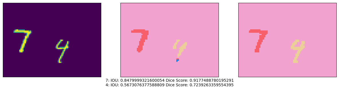
Visualize Predictions
# place a number here between 0 to 191 to pick an image from the test set
integer_slider = 105

ds = test_dataset.unbatch()
ds = ds.batch(200)
images = []

y_true_segments = []
for image, annotation in ds.take(2):
  y_true_segments = annotation
  images = image


iou, dice_score = class_wise_metrics(np.argmax(y_true_segments[integer_slider], axis=2), results[integer_slider])
show_annotation_and_prediction(image[integer_slider], annotation[integer_slider], results[integer_slider], iou, dice_score)
Compute IOU Score and Dice Score of your model
cls_wise_iou, cls_wise_dice_score = class_wise_metrics(np.argmax(y_true_segments, axis=3), results)

average_iou = 0.0
for idx, (iou, dice_score) in enumerate(zip(cls_wise_iou[:-1], cls_wise_dice_score[:-1])):
  print("Digit {}: IOU: {} Dice Score: {}".format(idx, iou, dice_score))
  average_iou += iou

grade = average_iou * 10

print("\nGrade is " + str(grade))

PASSING_GRADE = 60
if (grade>PASSING_GRADE):
  print("You passed!")
else:
  print("You failed. Please check your model and re-train")
Digit 0: IOU: 0.7597428676044692 Dice Score: 0.8634703189775721
Digit 1: IOU: 0.812731308135378 Dice Score: 0.8966925263417823
Digit 2: IOU: 0.6718855207544016 Dice Score: 0.8037458455304141
Digit 3: IOU: 0.6436363628292961 Dice Score: 0.7831858401104778
Digit 4: IOU: 0.6810783304830819 Dice Score: 0.8102874424505422
Digit 5: IOU: 0.5990493490856293 Dice Score: 0.7492568624328931
Digit 6: IOU: 0.7318317561823896 Dice Score: 0.8451534088918924
Digit 7: IOU: 0.6957992155646152 Dice Score: 0.8206150930821716
Digit 8: IOU: 0.6910964780121228 Dice Score: 0.8173353643601742
Digit 9: IOU: 0.6817821457399998 Dice Score: 0.8107853296777738

Grade is 69.68633334391383
You passed!
Save the Model
Once you’re satisfied with the results, you will need to save your model so you can upload it to the grader in the Coursera classroom. After running the cell below, please look for student_model.h5 in the File Explorer on the left and download it. Then go back to the Coursera classroom and upload it to the Lab item that points to the autograder of Week 3.
model.save("model.h5")
# You can also use this cell as a shortcut for downloading your model
from google.colab import files
files.download("model.h5")
<IPython.core.display.Javascript object>


<IPython.core.display.Javascript object>
Congratulations on completing this assignment on image segmentation!