Coursera
Image Segmentation with U-Net
Welcome to the final assignment of Week 3! You’ll be building your own U-Net, a type of CNN designed for quick, precise image segmentation, and using it to predict a label for every single pixel in an image - in this case, an image from a self-driving car dataset.
This type of image classification is called semantic image segmentation. It’s similar to object detection in that both ask the question: “What objects are in this image and where in the image are those objects located?,” but where object detection labels objects with bounding boxes that may include pixels that aren’t part of the object, semantic image segmentation allows you to predict a precise mask for each object in the image by labeling each pixel in the image with its corresponding class. The word “semantic” here refers to what’s being shown, so for example the “Car” class is indicated below by the dark blue mask, and “Person” is indicated with a red mask:

As you might imagine, region-specific labeling is a pretty crucial consideration for self-driving cars, which require a pixel-perfect understanding of their environment so they can change lanes and avoid other cars, or any number of traffic obstacles that can put peoples’ lives in danger.
By the time you finish this notebook, you’ll be able to:
- Build your own U-Net
- Explain the difference between a regular CNN and a U-net
- Implement semantic image segmentation on the CARLA self-driving car dataset
- Apply sparse categorical crossentropy for pixelwise prediction
Onward, to this grand and glorious quest!
Important Note on Submission to the AutoGrader
Before submitting your assignment to the AutoGrader, please make sure you are not doing the following:
- You have not added any extra
printstatement(s) in the assignment. - You have not added any extra code cell(s) in the assignment.
- You have not changed any of the function parameters.
- You are not using any global variables inside your graded exercises. Unless specifically instructed to do so, please refrain from it and use the local variables instead.
- You are not changing the assignment code where it is not required, like creating extra variables.
If you do any of the following, you will get something like, Grader not found (or similarly unexpected) error upon submitting your assignment. Before asking for help/debugging the errors in your assignment, check for these first. If this is the case, and you don’t remember the changes you have made, you can get a fresh copy of the assignment by following these instructions.
Table of Content
1 - Packages
Run the cell below to import all the libraries you’ll need:
import tensorflow as tf
import numpy as np

from tensorflow.keras.layers import Input
from tensorflow.keras.layers import Conv2D
from tensorflow.keras.layers import MaxPooling2D
from tensorflow.keras.layers import Dropout
from tensorflow.keras.layers import Conv2DTranspose
from tensorflow.keras.layers import concatenate

from test_utils import summary, comparator
2 - Load and Split the Data
import os
import numpy as np # linear algebra
import pandas as pd # data processing, CSV file I/O (e.g. pd.read_csv)

import imageio

import matplotlib.pyplot as plt
%matplotlib inline

path = ''
image_path = os.path.join(path, './data/CameraRGB/')
mask_path = os.path.join(path, './data/CameraMask/')
image_list = os.listdir(image_path)
mask_list = os.listdir(mask_path)
image_list = [image_path+i for i in image_list]
mask_list = [mask_path+i for i in mask_list]
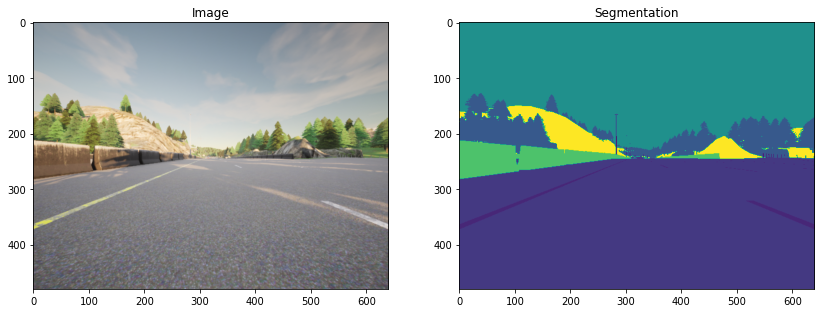
Check out the some of the unmasked and masked images from the dataset:
After you are done exploring, revert back to N=2. Otherwise the autograder will throw a list index out of range error.
N = 2
img = imageio.imread(image_list[N])
mask = imageio.imread(mask_list[N])
#mask = np.array([max(mask[i, j]) for i in range(mask.shape[0]) for j in range(mask.shape[1])]).reshape(img.shape[0], img.shape[1])

fig, arr = plt.subplots(1, 2, figsize=(14, 10))
arr[0].imshow(img)
arr[0].set_title('Image')
arr[1].imshow(mask[:, :, 0])
arr[1].set_title('Segmentation')
Text(0.5, 1.0, 'Segmentation')
2.1 - Split Your Dataset into Unmasked and Masked Images
image_list_ds = tf.data.Dataset.list_files(image_list, shuffle=False)
mask_list_ds = tf.data.Dataset.list_files(mask_list, shuffle=False)

for path in zip(image_list_ds.take(3), mask_list_ds.take(3)):
    print(path)
(<tf.Tensor: shape=(), dtype=string, numpy=b'./data/CameraRGB/000026.png'>, <tf.Tensor: shape=(), dtype=string, numpy=b'./data/CameraMask/000026.png'>)
(<tf.Tensor: shape=(), dtype=string, numpy=b'./data/CameraRGB/000027.png'>, <tf.Tensor: shape=(), dtype=string, numpy=b'./data/CameraMask/000027.png'>)
(<tf.Tensor: shape=(), dtype=string, numpy=b'./data/CameraRGB/000028.png'>, <tf.Tensor: shape=(), dtype=string, numpy=b'./data/CameraMask/000028.png'>)
image_filenames = tf.constant(image_list)
masks_filenames = tf.constant(mask_list)

dataset = tf.data.Dataset.from_tensor_slices((image_filenames, masks_filenames))

for image, mask in dataset.take(1):
    print(image)
    print(mask)
tf.Tensor(b'./data/CameraRGB/002128.png', shape=(), dtype=string)
tf.Tensor(b'./data/CameraMask/002128.png', shape=(), dtype=string)
2.2 - Preprocess Your Data
Normally, you normalize your image values by dividing them by 255. This sets them between 0 and 1. However, using tf.image.convert_image_dtype with tf.float32 sets them between 0 and 1 for you, so there’s no need to further divide them by 255.
def process_path(image_path, mask_path):
    img = tf.io.read_file(image_path)
    img = tf.image.decode_png(img, channels=3)
    img = tf.image.convert_image_dtype(img, tf.float32)

    mask = tf.io.read_file(mask_path)
    mask = tf.image.decode_png(mask, channels=3)
    mask = tf.math.reduce_max(mask, axis=-1, keepdims=True)
    return img, mask

def preprocess(image, mask):
    input_image = tf.image.resize(image, (96, 128), method='nearest')
    input_mask = tf.image.resize(mask, (96, 128), method='nearest')

    return input_image, input_mask

image_ds = dataset.map(process_path)
processed_image_ds = image_ds.map(preprocess)
3 - U-Net
U-Net, named for its U-shape, was originally created in 2015 for tumor detection, but in the years since has become a very popular choice for other semantic segmentation tasks.
U-Net builds on a previous architecture called the Fully Convolutional Network, or FCN, which replaces the dense layers found in a typical CNN with a transposed convolution layer that upsamples the feature map back to the size of the original input image, while preserving the spatial information. This is necessary because the dense layers destroy spatial information (the “where” of the image), which is an essential part of image segmentation tasks. An added bonus of using transpose convolutions is that the input size no longer needs to be fixed, as it does when dense layers are used.
Unfortunately, the final feature layer of the FCN suffers from information loss due to downsampling too much. It then becomes difficult to upsample after so much information has been lost, causing an output that looks rough.
U-Net improves on the FCN, using a somewhat similar design, but differing in some important ways. Instead of one transposed convolution at the end of the network, it uses a matching number of convolutions for downsampling the input image to a feature map, and transposed convolutions for upsampling those maps back up to the original input image size. It also adds skip connections, to retain information that would otherwise become lost during encoding. Skip connections send information to every upsampling layer in the decoder from the corresponding downsampling layer in the encoder, capturing finer information while also keeping computation low. These help prevent information loss, as well as model overfitting.
3.1 - Model Details

Contracting path (Encoder containing downsampling steps):
Images are first fed through several convolutional layers which reduce height and width, while growing the number of channels.
The contracting path follows a regular CNN architecture, with convolutional layers, their activations, and pooling layers to downsample the image and extract its features. In detail, it consists of the repeated application of two 3 x 3 unpadded convolutions, each followed by a rectified linear unit (ReLU) and a 2 x 2 max pooling operation with stride 2 for downsampling. At each downsampling step, the number of feature channels is doubled.
Crop function: This step crops the image from the contracting path and concatenates it to the current image on the expanding path to create a skip connection.
Expanding path (Decoder containing upsampling steps):
The expanding path performs the opposite operation of the contracting path, growing the image back to its original size, while shrinking the channels gradually.
In detail, each step in the expanding path upsamples the feature map, followed by a 2 x 2 convolution (the transposed convolution). This transposed convolution halves the number of feature channels, while growing the height and width of the image.
Next is a concatenation with the correspondingly cropped feature map from the contracting path, and two 3 x 3 convolutions, each followed by a ReLU. You need to perform cropping to handle the loss of border pixels in every convolution.
Final Feature Mapping Block: In the final layer, a 1x1 convolution is used to map each 64-component feature vector to the desired number of classes. The channel dimensions from the previous layer correspond to the number of filters used, so when you use 1x1 convolutions, you can transform that dimension by choosing an appropriate number of 1x1 filters. When this idea is applied to the last layer, you can reduce the channel dimensions to have one layer per class.
The U-Net network has 23 convolutional layers in total.
Important Note:
The figures shown in the assignment for the U-Net architecture depict the layer dimensions and filter sizes as per the original paper on U-Net with smaller images. However, due to computational constraints for this assignment, you will code only half of those filters. The purpose of showing you the original dimensions is to give you the flavour of the original U-Net architecture. The important takeaway is that you multiply by 2 the number of filters used in the previous step. The notebook includes all of the necessary instructions and hints to help you code the U-Net architecture needed for this assignment.
3.2 - Encoder (Downsampling Block)

The encoder is a stack of various conv_blocks:
Each conv_block() is composed of 2 Conv2D layers with ReLU activations. We will apply Dropout, and MaxPooling2D to some conv_blocks, as you will verify in the following sections, specifically to the last two blocks of the downsampling.
The function will return two tensors:
next_layer: That will go into the next block.skip_connection: That will go into the corresponding decoding block.
Note: If max_pooling=True, the next_layer will be the output of the MaxPooling2D layer, but the skip_connection will be the output of the previously applied layer(Conv2D or Dropout, depending on the case). Else, both results will be identical.
Exercise 1 - conv_block
Implement conv_block(...). Here are the instructions for each step in the conv_block, or contracting block:
- Add 2 Conv2D layers with
n_filtersfilters withkernel_sizeset to 3,kernel_initializerset to ‘he_normal’,paddingset to ‘same’ and ‘relu’ activation. - if
dropout_prob> 0, then add a Dropout layer with parameterdropout_prob - If
max_poolingis set to True, then add a MaxPooling2D layer with 2x2 pool size
# UNQ_C1
# GRADED FUNCTION: conv_block
def conv_block(inputs=None, n_filters=32, dropout_prob=0, max_pooling=True):
    """
    Convolutional downsampling block

    Arguments:
        inputs -- Input tensor
        n_filters -- Number of filters for the convolutional layers
        dropout_prob -- Dropout probability
        max_pooling -- Use MaxPooling2D to reduce the spatial dimensions of the output volume
    Returns:
        next_layer, skip_connection --  Next layer and skip connection outputs
    """

    ### START CODE HERE
    conv = Conv2D(filters = n_filters, # Number of filters
                  kernel_size = 3,   # Kernel size
                  activation = "relu",
                  padding = "same",
                  kernel_initializer = "he_normal")(inputs)
    conv = Conv2D(filters = n_filters, # Number of filters
                  kernel_size = 3,   # Kernel size
                  activation = "relu",
                  padding = "same",
                  kernel_initializer = "he_normal")(conv)
    ### END CODE HERE

    # if dropout_prob > 0 add a dropout layer, with the variable dropout_prob as parameter
    if dropout_prob > 0:
         ### START CODE HERE
        conv = Dropout(rate = dropout_prob)(conv)
         ### END CODE HERE


    # if max_pooling is True add a MaxPooling2D with 2x2 pool_size
    if max_pooling:
        ### START CODE HERE
        next_layer = MaxPooling2D(pool_size = (2, 2))(conv)
        ### END CODE HERE

    else:
        next_layer = conv

    skip_connection = conv

    return next_layer, skip_connection
input_size=(96, 128, 3)
n_filters = 32
inputs = Input(input_size)
cblock1 = conv_block(inputs, n_filters * 1)
model1 = tf.keras.Model(inputs=inputs, outputs=cblock1)

output1 = [['InputLayer', [(None, 96, 128, 3)], 0],
            ['Conv2D', (None, 96, 128, 32), 896, 'same', 'relu', 'HeNormal'],
            ['Conv2D', (None, 96, 128, 32), 9248, 'same', 'relu', 'HeNormal'],
            ['MaxPooling2D', (None, 48, 64, 32), 0, (2, 2)]]

print('Block 1:')
for layer in summary(model1):
    print(layer)

comparator(summary(model1), output1)

inputs = Input(input_size)
cblock1 = conv_block(inputs, n_filters * 32, dropout_prob=0.1, max_pooling=True)
model2 = tf.keras.Model(inputs=inputs, outputs=cblock1)

output2 = [['InputLayer', [(None, 96, 128, 3)], 0],
            ['Conv2D', (None, 96, 128, 1024), 28672, 'same', 'relu', 'HeNormal'],
            ['Conv2D', (None, 96, 128, 1024), 9438208, 'same', 'relu', 'HeNormal'],
            ['Dropout', (None, 96, 128, 1024), 0, 0.1],
            ['MaxPooling2D', (None, 48, 64, 1024), 0, (2, 2)]]

print('\nBlock 2:')
for layer in summary(model2):
    print(layer)

comparator(summary(model2), output2)
Block 1:
['InputLayer', [(None, 96, 128, 3)], 0]
['Conv2D', (None, 96, 128, 32), 896, 'same', 'relu', 'HeNormal']
['Conv2D', (None, 96, 128, 32), 9248, 'same', 'relu', 'HeNormal']
['MaxPooling2D', (None, 48, 64, 32), 0, (2, 2)]
[32mAll tests passed![0m
Block 2:
['InputLayer', [(None, 96, 128, 3)], 0]
['Conv2D', (None, 96, 128, 1024), 28672, 'same', 'relu', 'HeNormal']
['Conv2D', (None, 96, 128, 1024), 9438208, 'same', 'relu', 'HeNormal']
['Dropout', (None, 96, 128, 1024), 0, 0.1]
['MaxPooling2D', (None, 48, 64, 1024), 0, (2, 2)]
[32mAll tests passed
There are two new components in the decoder: up and merge. These are the transpose convolution and the skip connections. In addition, there are two more convolutional layers set to the same parameters as in the encoder.
Here you’ll encounter the Conv2DTranspose layer, which performs the inverse of the Conv2D layer. You can read more about it here.
Exercise 2 - upsampling_block
Implement upsampling_block(...).
For the function upsampling_block:
- Takes the arguments
expansive_input(which is the input tensor from the previous layer) andcontractive_input(the input tensor from the previous skip layer) - The number of filters here is the same as in the downsampling block you completed previously
- Your
Conv2DTransposelayer will taken_filterswith shape (3,3) and a stride of (2,2), with padding set tosame. It’s applied toexpansive_input, or the input tensor from the previous layer.
This block is also where you’ll concatenate the outputs from the encoder blocks, creating skip connections.
- Concatenate your Conv2DTranspose layer output to the contractive input, with an
axisof 3. In general, you can concatenate the tensors in the order that you prefer. But for the grader, it is important that you use[up, contractive_input]
For the final component, set the parameters for two Conv2D layers to the same values that you set for the two Conv2D layers in the encoder (ReLU activation, He normal initializer, same padding).
# UNQ_C2
# GRADED FUNCTION: upsampling_block
def upsampling_block(expansive_input, contractive_input, n_filters=32):
    """
    Convolutional upsampling block

    Arguments:
        expansive_input -- Input tensor from previous layer
        contractive_input -- Input tensor from previous skip layer
        n_filters -- Number of filters for the convolutional layers
    Returns:
        conv -- Tensor output
    """

    ### START CODE HERE
    up = Conv2DTranspose(
                 filters = n_filters,    # number of filters
                 kernel_size = (3, 3),    # Kernel size
                 strides = (2, 2),
                 padding = "same")(expansive_input)

    # Merge the previous output and the contractive_input
    merge = concatenate([up, contractive_input], axis=3)
    conv = Conv2D(filters = n_filters,   # Number of filters
                 kernel_size = 3,     # Kernel size
                 activation = "relu",
                 padding = "same",
                 kernel_initializer = "he_normal")(merge)
    conv = Conv2D(filters = n_filters,  # Number of filters
                 kernel_size = 3,   # Kernel size
                 activation = "relu",
                 padding = "same",
                 kernel_initializer = "he_normal")(conv)
    ### END CODE HERE

    return conv
input_size1=(12, 16, 256)
input_size2 = (24, 32, 128)
n_filters = 32
expansive_inputs = Input(input_size1)
contractive_inputs =  Input(input_size2)
cblock1 = upsampling_block(expansive_inputs, contractive_inputs, n_filters * 1)
model1 = tf.keras.Model(inputs=[expansive_inputs, contractive_inputs], outputs=cblock1)

output1 = [['InputLayer', [(None, 12, 16, 256)], 0],
            ['Conv2DTranspose', (None, 24, 32, 32), 73760],
            ['InputLayer', [(None, 24, 32, 128)], 0],
            ['Concatenate', (None, 24, 32, 160), 0],
            ['Conv2D', (None, 24, 32, 32), 46112, 'same', 'relu', 'HeNormal'],
            ['Conv2D', (None, 24, 32, 32), 9248, 'same', 'relu', 'HeNormal']]

print('Block 1:')
for layer in summary(model1):
    print(layer)

comparator(summary(model1), output1)
Block 1:
['InputLayer', [(None, 12, 16, 256)], 0]
['Conv2DTranspose', (None, 24, 32, 32), 73760]
['InputLayer', [(None, 24, 32, 128)], 0]
['Concatenate', (None, 24, 32, 160), 0]
['Conv2D', (None, 24, 32, 32), 46112, 'same', 'relu', 'HeNormal']
['Conv2D', (None, 24, 32, 32), 9248, 'same', 'relu', 'HeNormal']
[32mAll tests passed![0m
3.4 - Build the Model
This is where you’ll put it all together, by chaining the encoder, bottleneck, and decoder! You’ll need to specify the number of output channels, which for this particular set would be 23. That’s because there are 23 possible labels for each pixel in this self-driving car dataset.
Exercise 3 - unet_model
For the function unet_model, specify the input shape, number of filters, and number of classes (23 in this case).
For the first half of the model:
- Begin with a conv block that takes the inputs of the model and the number of filters
- Then, chain the first output element of each block to the input of the next convolutional block
- Next, double the number of filters at each step
- Beginning with
conv_block4, adddropout_probof 0.3 - For the final conv_block, set
dropout_probto 0.3 again, and turn off max pooling
For the second half:
- Use cblock5 as expansive_input and cblock4 as contractive_input, with
n_filters* 8. This is your bottleneck layer. - Chain the output of the previous block as expansive_input and the corresponding contractive block output.
- Note that you must use the second element of the contractive block before the max pooling layer.
- At each step, use half the number of filters of the previous block
conv9is a Conv2D layer with ReLU activation, He normal initializer,samepadding- Finally,
conv10is a Conv2D that takes the number of classes as the filter, a kernel size of 1, and “same” padding. The output ofconv10is the output of your model.
# UNQ_C3
# GRADED FUNCTION: unet_model
def unet_model(input_size=(96, 128, 3), n_filters=32, n_classes=23):
    """
    Unet model

    Arguments:
        input_size -- Input shape
        n_filters -- Number of filters for the convolutional layers
        n_classes -- Number of output classes
    Returns:
        model -- tf.keras.Model
    """
    inputs = Input(input_size)
    # Contracting Path (encoding)
    # Add a conv_block with the inputs of the unet_ model and n_filters
    ### START CODE HERE
    cblock1 = conv_block(inputs, n_filters)
    # Chain the first element of the output of each block to be the input of the next conv_block.
    # Double the number of filters at each new step
    cblock2 = conv_block(cblock1[0], n_filters * 2)
    cblock3 = conv_block(cblock2[0], n_filters * 4)
    cblock4 = conv_block(cblock3[0], n_filters * 8, dropout_prob = .3) # Include a dropout_prob of 0.3 for this layer
    # Include a dropout_prob of 0.3 for this layer, and avoid the max_pooling layer
    cblock5 = conv_block(cblock4[0], n_filters * 16, dropout_prob = .3, max_pooling=None)
    ### END CODE HERE

    # Expanding Path (decoding)
    # Add the first upsampling_block.
    # Use the cblock5[0] as expansive_input and cblock4[1] as contractive_input and n_filters * 8
    ### START CODE HERE
    ublock6 = upsampling_block(expansive_input = cblock5[0], contractive_input = cblock4[1], n_filters = n_filters * 8)
    # Chain the output of the previous block as expansive_input and the corresponding contractive block output.
    # Note that you must use the second element of the contractive block i.e before the maxpooling layer.
    # At each step, use half the number of filters of the previous block
    ublock7 = upsampling_block(expansive_input = ublock6, contractive_input = cblock3[1], n_filters = n_filters * 4)
    ublock8 = upsampling_block(expansive_input = ublock7, contractive_input = cblock2[1], n_filters = n_filters * 2)
    ublock9 = upsampling_block(expansive_input = ublock8, contractive_input = cblock1[1], n_filters = n_filters)
    ### END CODE HERE

    conv9 = Conv2D(n_filters,
                 3,
                 activation='relu',
                 padding='same',
                 kernel_initializer='he_normal')(ublock9)

    # Add a Conv2D layer with n_classes filter, kernel size of 1 and a 'same' padding
    ### START CODE HERE
    conv10 = Conv2D(filters = n_classes, kernel_size = 1, padding = "same")(conv9)
    ### END CODE HERE

    model = tf.keras.Model(inputs=inputs, outputs=conv10)

    return model
import outputs
img_height = 96
img_width = 128
num_channels = 3

unet = unet_model((img_height, img_width, num_channels))
comparator(summary(unet), outputs.unet_model_output)
[32mAll tests passed![0m
3.5 - Set Model Dimensions
img_height = 96
img_width = 128
num_channels = 3

unet = unet_model((img_height, img_width, num_channels))
Check out the model summary below!
unet.summary()
Model: "functional_9"
__________________________________________________________________________________________________
Layer (type)                    Output Shape         Param #     Connected to
==================================================================================================
input_6 (InputLayer)            [(None, 96, 128, 3)] 0
__________________________________________________________________________________________________
conv2d_26 (Conv2D)              (None, 96, 128, 32)  896         input_6[0][0]
__________________________________________________________________________________________________
conv2d_27 (Conv2D)              (None, 96, 128, 32)  9248        conv2d_26[0][0]
__________________________________________________________________________________________________
max_pooling2d_6 (MaxPooling2D)  (None, 48, 64, 32)   0           conv2d_27[0][0]
__________________________________________________________________________________________________
conv2d_28 (Conv2D)              (None, 48, 64, 64)   18496       max_pooling2d_6[0][0]
__________________________________________________________________________________________________
conv2d_29 (Conv2D)              (None, 48, 64, 64)   36928       conv2d_28[0][0]
__________________________________________________________________________________________________
max_pooling2d_7 (MaxPooling2D)  (None, 24, 32, 64)   0           conv2d_29[0][0]
__________________________________________________________________________________________________
conv2d_30 (Conv2D)              (None, 24, 32, 128)  73856       max_pooling2d_7[0][0]
__________________________________________________________________________________________________
conv2d_31 (Conv2D)              (None, 24, 32, 128)  147584      conv2d_30[0][0]
__________________________________________________________________________________________________
max_pooling2d_8 (MaxPooling2D)  (None, 12, 16, 128)  0           conv2d_31[0][0]
__________________________________________________________________________________________________
conv2d_32 (Conv2D)              (None, 12, 16, 256)  295168      max_pooling2d_8[0][0]
__________________________________________________________________________________________________
conv2d_33 (Conv2D)              (None, 12, 16, 256)  590080      conv2d_32[0][0]
__________________________________________________________________________________________________
dropout_3 (Dropout)             (None, 12, 16, 256)  0           conv2d_33[0][0]
__________________________________________________________________________________________________
max_pooling2d_9 (MaxPooling2D)  (None, 6, 8, 256)    0           dropout_3[0][0]
__________________________________________________________________________________________________
conv2d_34 (Conv2D)              (None, 6, 8, 512)    1180160     max_pooling2d_9[0][0]
__________________________________________________________________________________________________
conv2d_35 (Conv2D)              (None, 6, 8, 512)    2359808     conv2d_34[0][0]
__________________________________________________________________________________________________
dropout_4 (Dropout)             (None, 6, 8, 512)    0           conv2d_35[0][0]
__________________________________________________________________________________________________
conv2d_transpose_5 (Conv2DTrans (None, 12, 16, 256)  1179904     dropout_4[0][0]
__________________________________________________________________________________________________
concatenate_5 (Concatenate)     (None, 12, 16, 512)  0           conv2d_transpose_5[0][0]
                                                                 dropout_3[0][0]
__________________________________________________________________________________________________
conv2d_36 (Conv2D)              (None, 12, 16, 256)  1179904     concatenate_5[0][0]
__________________________________________________________________________________________________
conv2d_37 (Conv2D)              (None, 12, 16, 256)  590080      conv2d_36[0][0]
__________________________________________________________________________________________________
conv2d_transpose_6 (Conv2DTrans (None, 24, 32, 128)  295040      conv2d_37[0][0]
__________________________________________________________________________________________________
concatenate_6 (Concatenate)     (None, 24, 32, 256)  0           conv2d_transpose_6[0][0]
                                                                 conv2d_31[0][0]
__________________________________________________________________________________________________
conv2d_38 (Conv2D)              (None, 24, 32, 128)  295040      concatenate_6[0][0]
__________________________________________________________________________________________________
conv2d_39 (Conv2D)              (None, 24, 32, 128)  147584      conv2d_38[0][0]
__________________________________________________________________________________________________
conv2d_transpose_7 (Conv2DTrans (None, 48, 64, 64)   73792       conv2d_39[0][0]
__________________________________________________________________________________________________
concatenate_7 (Concatenate)     (None, 48, 64, 128)  0           conv2d_transpose_7[0][0]
                                                                 conv2d_29[0][0]
__________________________________________________________________________________________________
conv2d_40 (Conv2D)              (None, 48, 64, 64)   73792       concatenate_7[0][0]
__________________________________________________________________________________________________
conv2d_41 (Conv2D)              (None, 48, 64, 64)   36928       conv2d_40[0][0]
__________________________________________________________________________________________________
conv2d_transpose_8 (Conv2DTrans (None, 96, 128, 32)  18464       conv2d_41[0][0]
__________________________________________________________________________________________________
concatenate_8 (Concatenate)     (None, 96, 128, 64)  0           conv2d_transpose_8[0][0]
                                                                 conv2d_27[0][0]
__________________________________________________________________________________________________
conv2d_42 (Conv2D)              (None, 96, 128, 32)  18464       concatenate_8[0][0]
__________________________________________________________________________________________________
conv2d_43 (Conv2D)              (None, 96, 128, 32)  9248        conv2d_42[0][0]
__________________________________________________________________________________________________
conv2d_44 (Conv2D)              (None, 96, 128, 32)  9248        conv2d_43[0][0]
__________________________________________________________________________________________________
conv2d_45 (Conv2D)              (None, 96, 128, 23)  759         conv2d_44[0][0]
==================================================================================================
Total params: 8,640,471
Trainable params: 8,640,471
Non-trainable params: 0
__________________________________________________________________________________________________
3.6 - Loss Function
In semantic segmentation, you need as many masks as you have object classes. In the dataset you’re using, each pixel in every mask has been assigned a single integer probability that it belongs to a certain class, from 0 to num_classes-1. The correct class is the layer with the higher probability.
This is different from categorical crossentropy, where the labels should be one-hot encoded (just 0s and 1s). Here, you’ll use sparse categorical crossentropy as your loss function, to perform pixel-wise multiclass prediction. Sparse categorical crossentropy is more efficient than other loss functions when you’re dealing with lots of classes.
unet.compile(optimizer='adam',
              loss=tf.keras.losses.SparseCategoricalCrossentropy(from_logits=True),
              metrics=['accuracy'])
3.7 - Dataset Handling
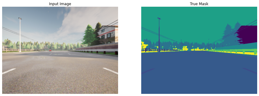
Below, define a function that allows you to display both an input image, and its ground truth: the true mask. The true mask is what your trained model output is aiming to get as close to as possible.
def display(display_list):
    plt.figure(figsize=(15, 15))

    title = ['Input Image', 'True Mask', 'Predicted Mask']

    for i in range(len(display_list)):
        plt.subplot(1, len(display_list), i+1)
        plt.title(title[i])
        plt.imshow(tf.keras.preprocessing.image.array_to_img(display_list[i]))
        plt.axis('off')
    plt.show()
for image, mask in image_ds.take(1):
    sample_image, sample_mask = image, mask
    print(mask.shape)
display([sample_image, sample_mask])
(480, 640, 1)
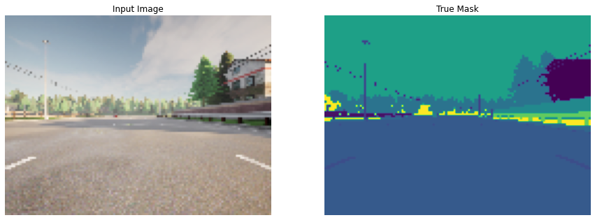
for image, mask in processed_image_ds.take(1):
    sample_image, sample_mask = image, mask
    print(mask.shape)
display([sample_image, sample_mask])
(96, 128, 1)
4 - Train the Model
EPOCHS = 40
VAL_SUBSPLITS = 5
BUFFER_SIZE = 500
BATCH_SIZE = 32
processed_image_ds.batch(BATCH_SIZE)
train_dataset = processed_image_ds.cache().shuffle(BUFFER_SIZE).batch(BATCH_SIZE)
print(processed_image_ds.element_spec)
model_history = unet.fit(train_dataset, epochs=EPOCHS)
(TensorSpec(shape=(96, 128, 3), dtype=tf.float32, name=None), TensorSpec(shape=(96, 128, 1), dtype=tf.uint8, name=None))
Epoch 1/40
34/34 [==============================] - 16s 457ms/step - loss: 1.7035 - accuracy: 0.4961
Epoch 2/40
34/34 [==============================] - 1s 40ms/step - loss: 0.9150 - accuracy: 0.7471
Epoch 3/40
34/34 [==============================] - 1s 40ms/step - loss: 0.6201 - accuracy: 0.8177
Epoch 4/40
34/34 [==============================] - 1s 39ms/step - loss: 0.5154 - accuracy: 0.8438
Epoch 5/40
34/34 [==============================] - 1s 39ms/step - loss: 0.4824 - accuracy: 0.8550
Epoch 6/40
34/34 [==============================] - 1s 41ms/step - loss: 0.3841 - accuracy: 0.8835
Epoch 7/40
34/34 [==============================] - 1s 43ms/step - loss: 0.3364 - accuracy: 0.8982
Epoch 8/40
34/34 [==============================] - 1s 39ms/step - loss: 0.3135 - accuracy: 0.9074
Epoch 9/40
34/34 [==============================] - 1s 39ms/step - loss: 0.2642 - accuracy: 0.9211
Epoch 10/40
34/34 [==============================] - 1s 39ms/step - loss: 0.2336 - accuracy: 0.9312
Epoch 11/40
34/34 [==============================] - 1s 40ms/step - loss: 0.2243 - accuracy: 0.9336
Epoch 12/40
34/34 [==============================] - 1s 40ms/step - loss: 0.2088 - accuracy: 0.9384
Epoch 13/40
34/34 [==============================] - 1s 40ms/step - loss: 0.1796 - accuracy: 0.9467
Epoch 14/40
34/34 [==============================] - 1s 39ms/step - loss: 0.1687 - accuracy: 0.9498
Epoch 15/40
34/34 [==============================] - 1s 39ms/step - loss: 0.1520 - accuracy: 0.9548
Epoch 16/40
34/34 [==============================] - 1s 40ms/step - loss: 0.1448 - accuracy: 0.9572
Epoch 17/40
34/34 [==============================] - 1s 40ms/step - loss: 0.1378 - accuracy: 0.9595
Epoch 18/40
34/34 [==============================] - 1s 39ms/step - loss: 0.1288 - accuracy: 0.9620
Epoch 19/40
34/34 [==============================] - 1s 39ms/step - loss: 0.1200 - accuracy: 0.9645
Epoch 20/40
34/34 [==============================] - 1s 39ms/step - loss: 0.1161 - accuracy: 0.9653
Epoch 21/40
34/34 [==============================] - 1s 39ms/step - loss: 0.1144 - accuracy: 0.9655
Epoch 22/40
34/34 [==============================] - 1s 40ms/step - loss: 0.1074 - accuracy: 0.9679
Epoch 23/40
34/34 [==============================] - 1s 40ms/step - loss: 0.1082 - accuracy: 0.9673
Epoch 24/40
34/34 [==============================] - 1s 39ms/step - loss: 0.1048 - accuracy: 0.9684
Epoch 25/40
34/34 [==============================] - 1s 39ms/step - loss: 0.0958 - accuracy: 0.9709
Epoch 26/40
34/34 [==============================] - 1s 39ms/step - loss: 0.0981 - accuracy: 0.9700
Epoch 27/40
34/34 [==============================] - 1s 39ms/step - loss: 0.0911 - accuracy: 0.9722
Epoch 28/40
34/34 [==============================] - 1s 39ms/step - loss: 0.0894 - accuracy: 0.9726
Epoch 29/40
34/34 [==============================] - 1s 39ms/step - loss: 0.0919 - accuracy: 0.9718
Epoch 30/40
34/34 [==============================] - 1s 39ms/step - loss: 0.0821 - accuracy: 0.9747
Epoch 31/40
34/34 [==============================] - 1s 40ms/step - loss: 0.0790 - accuracy: 0.9756
Epoch 32/40
34/34 [==============================] - 1s 39ms/step - loss: 0.0814 - accuracy: 0.9745
Epoch 33/40
34/34 [==============================] - 1s 39ms/step - loss: 0.0747 - accuracy: 0.9768
Epoch 34/40
34/34 [==============================] - 1s 39ms/step - loss: 1.7368 - accuracy: 0.5141
Epoch 35/40
34/34 [==============================] - 1s 39ms/step - loss: 1.0071 - accuracy: 0.7425
Epoch 36/40
34/34 [==============================] - 1s 39ms/step - loss: 0.5808 - accuracy: 0.8433
Epoch 37/40
34/34 [==============================] - 1s 39ms/step - loss: 0.4775 - accuracy: 0.8688
Epoch 38/40
34/34 [==============================] - 1s 39ms/step - loss: 0.4331 - accuracy: 0.8794
Epoch 39/40
34/34 [==============================] - 1s 39ms/step - loss: 0.4589 - accuracy: 0.8714
Epoch 40/40
34/34 [==============================] - 1s 39ms/step - loss: 0.3854 - accuracy: 0.8876
4.1 - Create Predicted Masks
Now, define a function that uses tf.argmax in the axis of the number of classes to return the index with the largest value and merge the prediction into a single image:
def create_mask(pred_mask):
    pred_mask = tf.argmax(pred_mask, axis=-1)
    pred_mask = pred_mask[..., tf.newaxis]
    return pred_mask[0]
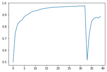
4.2 - Plot Model Accuracy
Let’s see how your model did!
plt.plot(model_history.history["accuracy"])
[<matplotlib.lines.Line2D at 0x7fe6ec23c6a0>]
4.3 - Show Predictions
Next, check your predicted masks against the true mask and the original input image:
def show_predictions(dataset=None, num=1):
    """
    Displays the first image of each of the num batches
    """
    if dataset:
        for image, mask in dataset.take(num):
            pred_mask = unet.predict(image)
            display([image[0], mask[0], create_mask(pred_mask)])
    else:
        display([sample_image, sample_mask,
             create_mask(unet.predict(sample_image[tf.newaxis, ...]))])
show_predictions(train_dataset, 6)
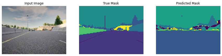
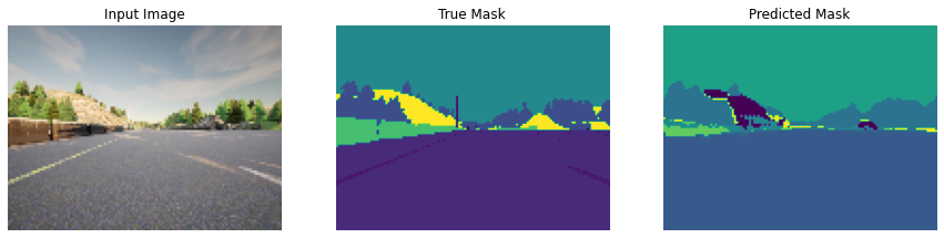
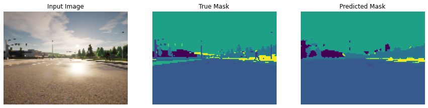
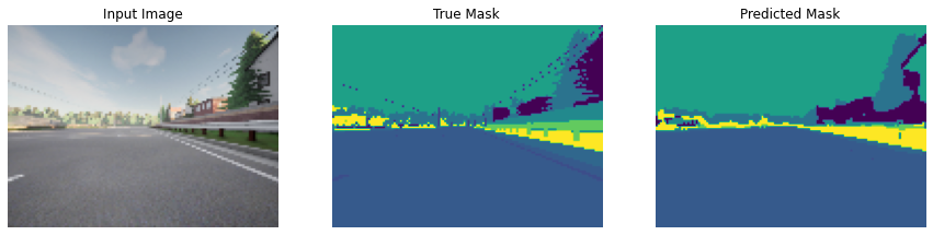
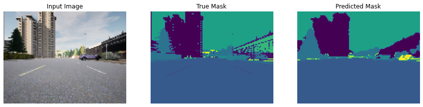
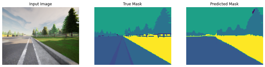
With 40 epochs you get amazing results!
Free Up Resources for Other Learners
In order to provide our learners a smooth learning experience, please free up the resources used by your assignment by running the cell below so that the other learners can take advantage of those resources just as much as you did. Thank you!
Note:
- Run the cell below when you are done with the assignment and are ready to submit it for grading.
- When you’ll run it, a pop up will open, click
Ok. - Running the cell will
restart the kernel.
%%javascript
IPython.notebook.save_checkpoint();
if (confirm("Clear memory?") == true)
{
    IPython.notebook.kernel.restart();
}
<IPython.core.display.Javascript object>
Conclusion
You’ve come to the end of this assignment. Awesome work creating a state-of-the art model for semantic image segmentation! This is a very important task for self-driving cars to get right. Elon Musk will surely be knocking down your door at any moment. ;)
What you should remember:
- Semantic image segmentation predicts a label for every single pixel in an image
- U-Net uses an equal number of convolutional blocks and transposed convolutions for downsampling and upsampling
- Skip connections are used to prevent border pixel information loss and overfitting in U-Net